6 Diffraction and interference
Again, we will briefly look at definitions. Let’s start with interference:
- The superposition of two (or more) waves to produce a new wave1.
- A phenomenon in which two coherent waves are combined by adding their intensities or displacements with due consideration for their phase difference2.
1 Google AI
2 Wikipedia
In this course, we focus on waves that follow a linear wave equation, so that given two solutions to the equation, the sum is also a solution. Hence, given two sources, the resulting wave is that obtained by solving the equation for each source individually and then simply summing the results. The resulting interaction between the two waves is then referred to as interference.
What about diffraction:
- The spreading of waves as they pass through an opening or around an obstacle3.
- The deviation of waves from straight-line propagation without any change in their energy due to an obstacle or through an aperture4.
3 Google AI
4 Wikipedia
5 In our analysis, infinitely many sources.
But it turns out that diffraction is essentially just interference, but with very many5 sources. You are hopefully familiar with the basic double-slit experiment, simplified so that each slit is considered as a single source. To calculate the interference pattern, we apply the principle of superposition to the wave from the two sources, i.e. we sum the waves. For three slits, we would sum three waves. For one thousand slits, we sum one thousand waves. Now what happens if we moves these slits so that they are positioned next to each other, with no gaps. We continue to sum the waves. However, now the slits have merged to become a single aperture and, according to the definitions above, the resulting wave is the result of diffraction.
6.1 The Huygens-Fresnel principle
The Huygens-Fresnel principle states that
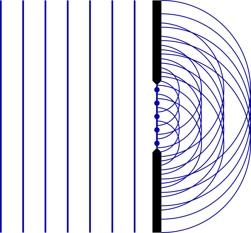
- Every point of a wavefront serves as a source of secondary spherical wavelets. The resulting wave is calculated by the superposition of these wavelets.
This is illustrated in figure 6.1 where five secondary sources are placed on the wavefront within the aperture.
6.2 Spherical waves
Given that the Huygens-Fresnel principle involves spherical waves and the following analyses will involve superposing such waves, we should ensure that we know the formula for such waves. Recall the wave equation \[ \nabla^2E = \frac{1}{v^2}\frac{\partial^2E}{\partial t^2}. \] I will claim that \[ E = \frac{f(r - vt)}{r} \] is a solution, where \(r\) is the distance from the origin6. You should check that this solution does indeed satisfy the wave equation. It will be useful to know that, in spherical coordinates \[ \nabla^2E = \frac{1}{r^2}\frac{\partial}{\partial r}\left(r^2\frac{\partial E}{\partial r}\right) + \frac{1}{r^2\sin\theta}\frac{\partial}{\partial\theta}\left(\sin\theta\frac{\partial E}{\partial\theta}\right) + \frac{1}{r^2\sin^2\theta}\frac{\partial^2E}{\partial\phi^2}. \]
6 Of course, \(r\) can be the distance from any point we choose — spherical waves are not all required to spread out from the origin.
6.3 Fresnel and Fraunhofer diffraction
In what follows, we will consider what happens to light when it encounters an opaque barrier with one or more apertures or slits. The study of the result diffraction patterns is often split into two domains:
Fresnel diffraction: Also called near-field diffraction, Fresnel diffraction concerns the situation when either the light source or the screen (or both) are ‘close’ to the barrier.
Fraunhofer diffraction: Also called far-field diffraction, Fraunhofer diffraction concerns the situation where both light source and screen are ‘far’ from the barrier.
The diffraction pattern changes as the distance from the barrier increases but eventually settles into the Fraunhofer pattern, after which the size of the pattern changes but the shape does not. Fresnel diffraction is typically more difficult to calculate, requiring the analysis of multiple spherical waves, while the large distances associated with Fraunhofer diffraction mean that simplifying assumptions can be made7. We will therefore focus on Fraunhofer diffraction for the reminder of this chapter.
7 We can consider wavefronts to be effectively planar.
Note that Fresnel and Fraunhofer diffraction are not different effects. They merely refer to examining the effect of diffraction, but at different distances from the barrier.
There remains the question of what we mean by ‘close’ or ‘far’ in our definitions. The calculation of Fraunhofer diffraction requires simplifying mathematical assumptions that are not valid too close to the screen. We will see that the domain in which these assumptions make sense depends both on the aperture width and the wavelength. We will find that Fraunhofer diffraction is valid provided both source and screen are at least a distance of \(R\) from the screen, where \(R = a^2/\lambda\) and where \(a\) is the slit width and \(\lambda\) is the wavelength.
6.4 Single-slit diffraction
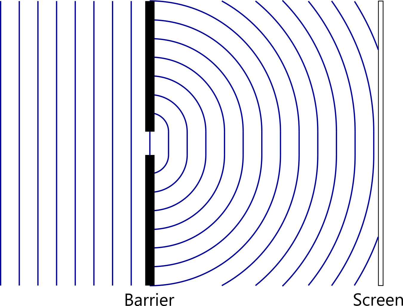
The setup is as shown in figure 6.2, but with the screeen further from the barrier than shown. Waves approach the barrier from the left. These are plane waves8, monochromatic9 and coherent10. To begin, we will consider the situation in two dimensions only. In this case, the aperture can be considered as a line of sources of spherical wavelets which we will superpose to determine the diffraction pattern.
8 Suggesting a source of light infinitely far away.
9 A single frequency (and wavelength).
10 The same phase.
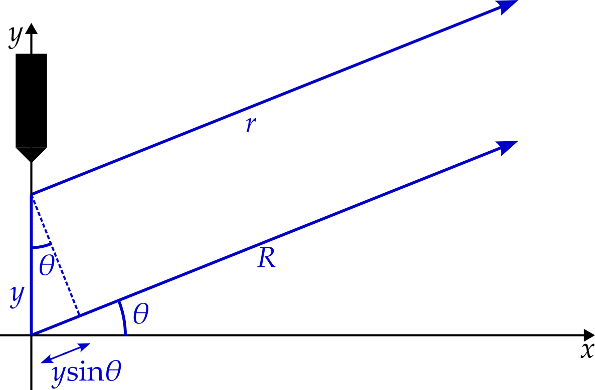
Consider a fixed point, \(P\), on the screen such that a wavelet starting at the aperture centre must travel a distance \(R\) at angle \(\theta\) to the horizontal to reach it. Wavelets starting from other locations within the aperture travel a slightly different distance to reach \(P\), as shown in figure 6.3. The difference in distances will determine whether the wavelets interfere constructively or destructively.
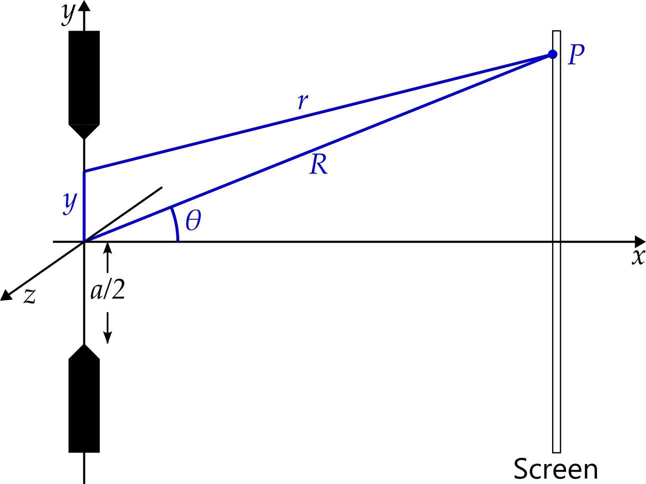
Using the cosine rule11 we find that \[ r = R\sqrt{1 - 2\frac{y}{R}\sin\theta + \frac{y^2}{R^2}}. \] We Taylor expand in \(y/R\) to get \[ r = R - y\sin\theta + \frac{y^2}{2R}\cos^2\theta + \ldots \] We would like to be able to ignore the third term. How small must it be to allow us to disregard it? It must be small compared with the wavelength, otherwise omitting the term will make a significant difference to the way the wavelets interfere at point \(P\). That is, we want \(y^2/R \ll \lambda\). Noting that \(y\) might be as large as \(a/2\) and rearranging this condition, we find that we require \(R \gg a^2/\lambda\), as mentioned earlier.
11 To remind you, this states that if \(a\), \(b\) and \(c\) are the lengths of the three sides of a triangle and \(A\) is the angle opposite side \(a\) then \[ a^2 = b^2 + c^2 - 2bc\cos A. \]
Ignoring this term, we find that the difference in path lengths is \(y\sin\theta\). Interestingly, this is what we would get if we simply assumed that the rays were parallel, as shown in figure 6.4.
We now sum the contribution of all the wavelets at position \(P\). Since we consider contributions from all the positions within the aperture, this is actually an integral. We get \[ E = A\int_{-a/2}^{a/2}\frac{e^{i\left(k\left(R - y\sin\theta\right) - \omega t\right)}}{R - y\sin\theta}\,dy. \] The \(y\sin\theta\) in the denominator is rather awkward. However, for large \(R\) and small \(y\), its contribution is negligible12 while the change \(y\sin\theta\) makes to the phase of the wave is not. We therefore ignore the \(y\sin\theta\) in the denominator and get \[ E = \frac{A}{R}e^{i\left(kR-\omega t\right)}\int_{a/2}^{a/2}e^{-iky\sin\theta}\,dy. \] We can do this integral. \[ \begin{aligned} \int_{a/2}^{a/2}e^{-iky\sin\theta}\,dy &= \frac{i}{k\sin\theta}\left[e^{-iky\sin\theta}\right]_{-a/2}^{a/2}\\ &= \frac{i}{k\sin\theta}\left(e^{-\frac{1}{2}ika\sin\theta} - e^{\frac{1}{2}ika\sin\theta}\right). \end{aligned} \] If we let \[ \beta = \frac{1}{2}ka\sin\theta \] then this is \[ \begin{aligned} \int_{a/2}^{a/2}e^{-iky\sin\theta}\,dy &= \frac{ai}{2\beta}\left(e^{-i\beta} - e^{i\beta}\right)\\ &= \frac{ai}{2\beta}\left(-2i\sin\beta\right)\\ &= \frac{a\sin\beta}{\beta}. \end{aligned} \] We therefore get \[ E = \frac{Aa}{R}\frac{\sin\beta}{\beta}e^{i\left(kR-\omega t\right)}. \]
12 We note that \[ \frac{1}{R-y\sin\theta} \simeq \frac{1}{R} + \frac{y}{R^2}\sin\theta. \]
13 Being physicists, we say that \(\sin \theta / \theta = 1\). A mathematician might say that this is undefined, being zero divided by zero, but would be happy to agree that the limit, as theta approaches zero, is one.
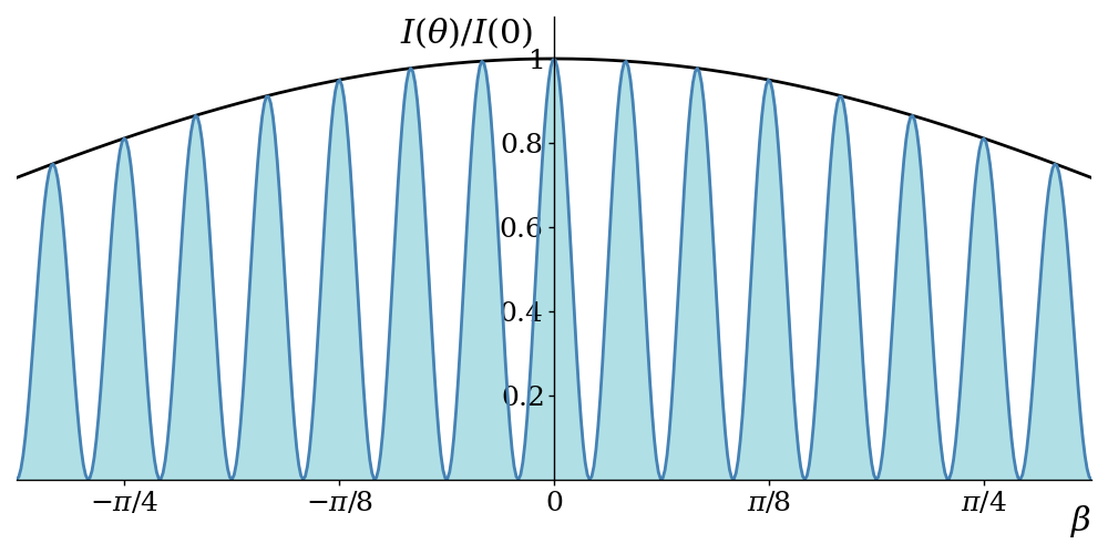
Now recall that the intensity is proportional to the amplitude squared. If \(I(\theta)\) represents the light intensity at angle \(\theta\), then we find that \(I(0)\) is proportional to13 \((Aa/R)^2\). We then find that, for any \(\theta\) \[ I(\theta) = I(0)\frac{\sin^2\beta}{\beta^2}. \] A plot of this function is shown in figure 6.5.
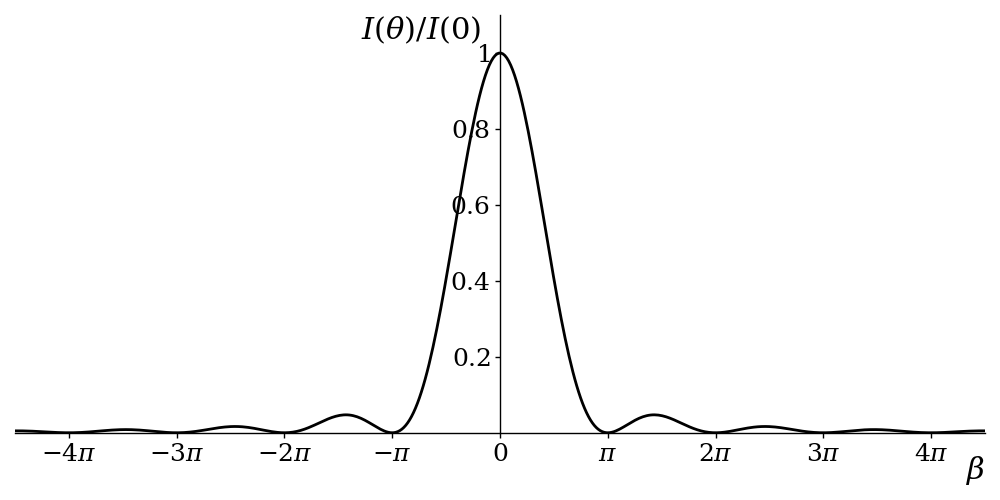
We see that minima occur whenever \(\beta\) is a multiple of \(\pi\), except at the central peak at \(\beta = 0\). Other maxima occur at \(\beta\) approximately equal to \(\pm1.43\pi\), \(\pm2.46\pi\), \(\pm3.47\pi\), etc.
By differentiating the intensity with respect to \(\beta\), find a simple equation satisfied by the value of \(\beta\) at the maxima of intensity. Confirm that the values for \(\beta\) listed above satisfy this equation.
Noting that \[ \beta = \frac{\pi a}{\lambda}\sin\theta \] we see that when the slit width is large compared to the wavelength then \(\beta\) increases rapidly as \(\theta\) is increased. As a result, the central peak is very narrow14 and light intensity is negligible except when \(\theta\) is close to zero. There is little spreading of the waves, or in other words, little diffraction. In contrast, when the slit width is small compared with the wavelength, \(\beta\) increases very slowly as \(\theta\) increases. As a result, \(\theta\) reaches an angle of \(\pi / 2\) before \(\beta\) leaves the central peak of the illustrated graph15. The light is spread almost equally across all values of \(\theta\). Finally, when the slit width and the wavelength are similar, we see bands of light, i.e. a diffraction pattern, as suggested by the graph.
14 Imagine the graph squashed horizontally.
15 Imagine the graph stretched horizontally.
6.4.1 In three dimensions
Thus far we have considered the slit as an idealised line source16 in two dimensions. However, you may have noticed the inclusion of the \(z\) axis in figure 6.3. How much light is detected at non-zero values of \(z\)? The key here is to notice that if we consider the aperture as simply an idealised line source of light, then there is rotational symmetry around the \(y\)-axis. Hence, for a line source that is long compared with the wavelength, the intensity of light is negligible except in the \(x\)-\(z\) plane, where \(\theta\) is close to zero. This is equivalent to a single light source at the centre, but one which only emits light in the \(x\)-\(z\) plane, i.e. circular waves. If the line source is very short compared with the wavelength, it is equivalent to a single light source that emits light in all directions, i.e. spherical waves.
16 A line of zero thickness, each point of which is emitting monochromatic coherent spherical waves.
We must also revisit the notion of the aperture as a idealised line source. Figure 6.6 shows a slit in a barrier in three dimensions. This slit has both length and width. Start by thinking of the slit a collection of vertical idealised line sources. Since the length of the slit is much larger than the wavelength of the light, the light from each line source does not diffract much in the vertical direction. Each vertical line can be thought of as equivalent to a source of light, positioned at mid-height within the slit, emitting light only in the horizontal plane.
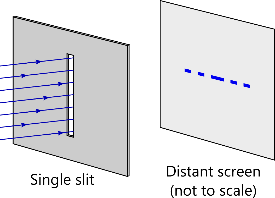
This now means that we have a short horizontal row of line sources. The width of the slit is not large compared with the wavelength and so light diffracts horizontally. The result is the diffraction pattern shown on the screen.
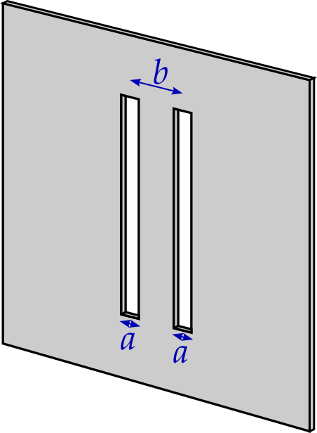
6.5 Double-slit diffraction
Moving to two slits is now straightforward. Consider two slits, both of width \(a\) as before, with centres separated by \(b\), as shown in figure 6.7.
Each slit is displaced by \(b/2\) from the centre. Recall that a centrally placed slit gives us \[ E = \frac{Aa}{R}\frac{\sin\beta}{\beta}e^{i\left(kR-\omega t\right)}. \] Using the same logic as for the single slit case, a slit displaced by \(b/2\) produces \[ E = \frac{Aa}{R}\frac{\sin\beta}{\beta}e^{i\left(kR-\omega t \pm \alpha\right)} \] where \[ \alpha = \frac{1}{2}kb\sin\theta. \] Summing the waves from the two sources produces \[ \begin{aligned} E &= \frac{Aa}{R}\frac{\sin\beta}{\beta}e^{i\left(kR-\omega t - \alpha\right)} + \frac{Aa}{R}\frac{\sin\beta}{\beta}e^{i\left(kR-\omega t + \alpha\right)}\\ &= \frac{Aa}{R}\frac{\sin\beta}{\beta}e^{i\left(kR-\omega t\right)}\left(e^{i\alpha} + e^{-i\alpha}\right)\\ &= \frac{2Aa}{R}\frac{\sin\beta}{\beta}e^{i\left(kR-\omega t\right)}\cos\alpha. \end{aligned} \] The intensity is now given by17 \[ I(\theta) = I(0)\left(\frac{\sin^2\beta}{\beta^2}\right)\cos^2\alpha. \]
17 The intensity at \(\theta = 0\) is now four times what it was for a single slit. (I.e. this is a different \(I(0)\).)
Setting \(b = 3a\), this produces the graph shown in figure 6.8.
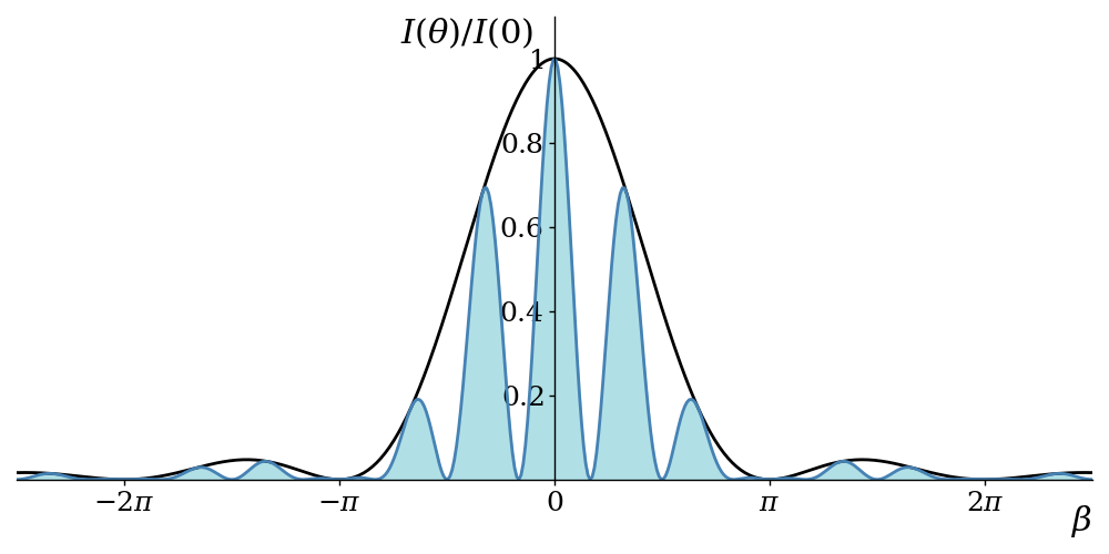
The black curve here ignores the factor of \(\cos^2\alpha\) and is the same shape as that from the single-slit experiment. The cosine part of the formula oscillates more rapidly18. Multiplying the two parts produces the blue curve.
18 Since \(\alpha = 3\beta\) in this case.
Notice that where we would expect the third peak from the centre to appear, at \(\beta = \pm\pi\), the peak has been squashed by the black curve. If we make the slits narrower but maintain the slit separation, then we stretch the black curve horizontally and obtain a more familiar interference pattern with bands of similar intensity, as shown in figure 6.9.