4  Electromagnetic waves, reflection and refraction

In this chapter we will start by considering the nature of electromagnetic waves and examine a few of their properties. We then analyse the reflection and refraction that occurs as light impacts upon a surface between two transparent materials. We will discover that the polarisation of the light has a significant impact upon the results.

4.1 On the nature of electromagnetic waves

Thus¹ far, we have considered waves travelling through a medium that is displaced by the wave, e.g. waves on a string. In contrast, when considering light travelling through the vacuum there is no material to displace. Nothing is moving. Instead, we have fluctuations in the electromagnetic field.

¹ In this section, we will be forced to encounter a number of results from electromagnetism. For now, you will have to trust me a little, but do look back at these notes after completing electromagnetism.

In the appendix, it is shown that in the absence of electric charges or currents, both the electric, \(\mathbf{E}\), and magnetic, \(\mathbf{B}\), components of the electromagnetic field satisfy the wave equation in three dimensions. It is also shown that for plane waves, travelling in the \(x\) direction, \(\mathbf{E}_x = \mathbf{B}_x = 0\), i.e. the waves are transverse. Notice again that nothing is moving here. If we consider just the electric field, the electric field is merely changing not moving.

The appendix also shows that the magnetic field, \(\mathbf{B}\), is oriented perpendicular to both the propagation of the wave and the resulting electric field. If the wave propagates in the \(x\) direction then the magnetic field is given by² \[ \mathbf{B} = \frac{k}{\omega}\hat{\mathbf{x}}\times\mathbf{E} = \frac{1}{v}\hat{\mathbf{x}}\times\mathbf{E}. \tag{4.1}\]

² Later, we will consider light travelling through a medium, e.g. air, water or glass, so I will use \(v\) rather than \(c\) for the wave’s velocity.

This is illustrated graphically in figure 1.

Figure 4.1: A vertically polarised electromagnetic wave. (The direction of the polarisation is given by the electric field.) Note that the graph does not plot displacements, but the value of the electric and magnetic field vectors at each point on the \(x\)-axis.

4.2 Energy and intensity

The energy density of an electromagnetic field is given by³ \[ u = \frac{1}{2}\left(\epsilon E^2 + \frac{1}{\mu}B^2\right) \] For the sinusoidal plane wave, we can use equation 4.1 to see that \[ B^2 = \frac{1}{v^2}E^2 \] while the velocity of the wave is given by⁴ \[ v = \frac{1}{\sqrt{\mu\epsilon}} \tag{4.2}\] and so the electric and magnetic fields’ contribution to the energy are equal and we have \[ u = \epsilon E^2. \] For the plane wave given by \[ \begin{aligned} \mathbf{E}(x, t) &= \mathbf{E}^0\sin\left(kx - \omega t + \delta\right),\\ \mathbf{B}(x, t) &= \mathbf{B}^0\sin\left(kx - \omega t + \delta\right) \end{aligned} \] we therefore get \[ u = \epsilon \left(\mathbf{E}^0\right)^2\sin^2\left(kx - \omega t + \delta\right). \]

³ Here \(\epsilon\) is called the permitivity of the medium, while \(\mu\) is the permeability. You will learn more about these and the derivation of this formula in the electromagnetism section of the unit.

⁴ See the appendix.

⁵ The energy transported per unit area, per unit time. This is naturally a vector quantity, giving the direction in which energy is transported.

⁶ Again, to be seen later in the unit.

Given a travelling wave such as this one, the wave carries the energy with it. The energy flux density⁵ is given by the Poynting vector⁶ \[ \mathbf{S} = \frac{1}{\mu}(\mathbf{E}\times\mathbf{B}). \] Calculating this for the plane wave travelling in the \(x\) direction, we get \[ \mathbf{S} = v\epsilon \left(\mathbf{E}^0\right)^2\sin^2\left(kx - \omega t + \delta\right)\hat{\mathbf{x}} = vu\hat{\mathbf{x}}, \] as we might expect.

Notice that both the energy and the energy transfer, at a fixed point in the wave, is a varying quantity. Also, the frequency of visible light is between 400 and 790 terahertz, i.e. at least 400 trillion oscillations per second. to get quantities of more day-to-day relevance, we take the time average of these quantities, i.e. \[ \left<u\right> = \frac{1}{2}\epsilon\left(E^0\right)^2, \qquad \left<\mathbf{S}\right> = \frac{1}{2}v\epsilon\left(E^0\right)^2\hat{\mathbf{x}} \] The intensity is then \[ I = \left<S\right> = \frac{1}{2}v\epsilon\left(E^0\right)^2. \]

4.3 Reflection and refraction

Let’s consider what happens when a planar electromagnetic wave encounters the surface between two transparent media, e.g. light striking the surface of a lake. In each of the media, we simply have waves satisfying the wave equation. At the boundary between air and water, the fields must satisfy the following boundary conditions⁷ \[ \begin{aligned} \epsilon_1E_1^\perp &= \epsilon_2E_2^\perp, & \mathbf{E}_1^\parallel &= \mathbf{E}_2^{\parallel}\\ B_1^\perp &= B_2^\perp, & \frac{1}{\mu_1}\mathbf{B}_1^\parallel &= \frac{1}{\mu_2}\mathbf{B_2}^\parallel. \end{aligned} \] Here the electric and magnetic fields just to the left of the boundary, in medium 1, and just to the right of the boundary, in medium 2, are related. \(E^\perp\) refers to the component of the electric field normal to the boundary, while \(\mathbf{E}^\parallel\) refers to the components parallel to it.

⁷ Again, you will need to understand a good amount of electromagnetism derive these boundary conditions. They can be found in section 7.3.6 of Introduction to Electrodynamics, by David J. Griffiths.

Note that the velocity of the wave will be different in each of the two media. If \(c\) is the speed of light in a vacuum and \(v\) is the speed in a medium, then the medium’s refractive index is \[ n = \frac{c}{v}. \]

4.3.1 Normal incidence

We will start with the simplest case, where the propagation of the incident wave is at right angles to the boundary.

Figure 4.2: A planar electromagnetic wave strikes the boundary between two transparent media, with the direction of propagation of the incident wave at right angles to the boundary. We see the incident wave, the reflected wave and the transmitted wave.

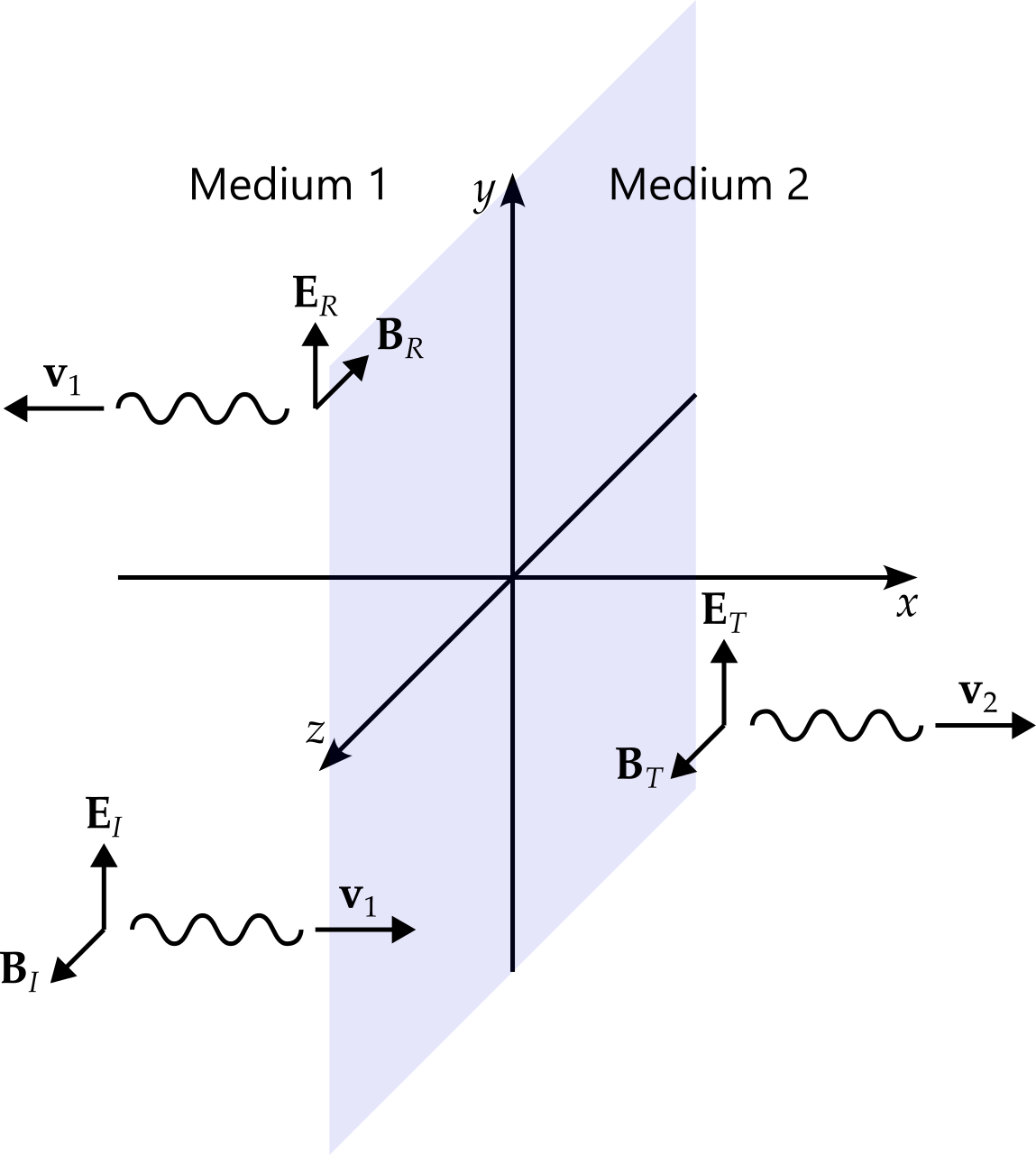
working with the complex representation, the incident wave is given by \[ \begin{aligned} \mathbf{E}_I &= E^0_Ie^{i\left(k_1x - \omega t\right)}\hat{\mathbf{y}},\\ \mathbf{B}_I &= \frac{1}{v_1}E^0_Ie^{i\left(k_1x - \omega t\right)}\hat{\mathbf{z}}, \end{aligned} \] the reflected wave by \[ \begin{aligned} \mathbf{E}_R &= E^0_Re^{i\left(-k_1x - \omega t\right)}\hat{\mathbf{y}},\\ \mathbf{B}_R &= -\frac{1}{v_1}E^0_Re^{i\left(-k_1x - \omega t\right)}\hat{\mathbf{z}}, \end{aligned} \] and the transmitted wave by \[ \begin{aligned} \mathbf{E}_T &= E^0_Te^{i\left(k_2x - \omega t\right)}\hat{\mathbf{y}},\\ \mathbf{B}_T &= \frac{1}{v_2}E^0_Re^{i\left(k_2x - \omega t\right)}\hat{\mathbf{z}}, \end{aligned} \]

We now check the boundary conditions at \(x = 0\). Neither the electric nor the magnetic fields have a component perpendicular to the surface. This leaves only the equations relating the components parallel to the surface. For the electric fields, this gives \[ E^0_Ie^{-i\omega t} + E^0_Re^{-i\omega t} = E^0_Te^{-i\omega t} \] and hence \[ E^0_I + E^0_R = E^0_T, \tag{4.3}\] while for the magnetic fields we get \[ \frac{1}{\mu_1v_1}E^0_Ie^{-i\omega t} - \frac{1}{\mu_1 v_1}E^0_Re^{-i\omega t} = \frac{1}{\mu_2 v_2}E^0_Re^{-i\omega t} \] and hence \[ \frac{1}{\mu_1v_1}E^0_I - \frac{1}{\mu_1 v_1}E^0_R = \frac{1}{\mu_2 v_2}E^0_T, \] which can be written as \[ E^0_I - E^0_R = \beta E^0_T, \tag{4.4}\] where \[ \beta = \frac{\mu_1v_1}{\mu_2v_2} = \frac{\mu_1n_2}{\mu_2n_1} \] and \(n_1\), \(n_2\) are the refractive indices of the two media.

Equations 4.3 and 4.4 are easily solved to find \(E^0_R\) and \(E^0_T\) in terms of \(E^0_T\). We get \[ E^0_R = \frac{1 - \beta}{1 + \beta}E^0_I, \qquad E^0_T = \frac{2}{1+\beta}E^0_I. \] If⁸ \(\mu_1 = \mu_2\), then this becomes \[ E^0_R = \frac{v_2 - v_1}{v_2 + v_1}E^0_I, \qquad E^0_T = \frac{2v_2}{v_2 + v_1}E^0_I \] and in terms of the refractive indices, this is \[ E^0_R = \frac{n_1 - n_2}{n_1 + n_2}E^0_I, \qquad E^0_T = \frac{2n_1}{n_1 + n_2}E^0_I. \]

⁸ Permeabilities \(\mu_1\) and \(\mu_2\) are usually similar to that of the vacuum, \(\mu_0\), so this is usually a good approximation.

Hence if \(v_2 > v_1\) (e.g. water to air) then the reflected wave is right side up, while if \(v_2 < v_1\) (e.g. air to water), then the reflected wave is flipped.

We can use this result to find how much energy is transmitted and how much is reflected. Remembering that the intensity is \[ I = \frac{1}{2}\epsilon v\left(E^0\right)^2 \] we calculate the reflection coefficient \[ R = \frac{I_R}{I_I} = \left(\frac{E^0_R}{E^0_I}\right)^2 = \left(\frac{v_2 - v_1}{v_2 + v_1}\right)^2 = \left(\frac{n_1 - n_2}{n_1 + n_2}\right)^2 \] and the transmission coefficient \[ T = \frac{I_T}{I_I} = \frac{\epsilon_2v_2}{\epsilon_1v_1}\left(\frac{E^0_T}{E^0_I}\right)^2 = \frac{4v_2v_2}{\left(v_1 + v_2\right)^2} = \frac{4n_1n_2}{\left(n_1 + n_2\right)^2}. \]

4.3.2 Oblique incidence (part 1)

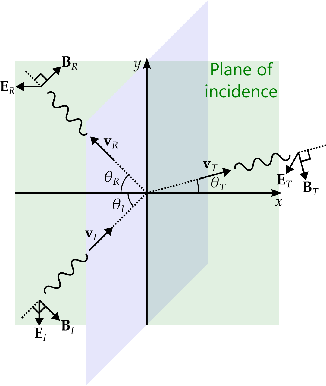
We now proceed to the more complex case of oblique incidence. We start by defining the plane of incidence to be the plane that contains the incident ray⁹ and the line perpendicular to the surface. This is illustrated in green in figure 4.3¹⁰.

⁹ Actually, we consider entire plane waves striking the surface and hence a collection of rays. However, for each incident ray, the plane of incidence will be parallel to that for any other ray. It is this orientation of the plane, rather than its placement, that is of importance here.

¹⁰ This figure assumes that the velocity of all three waves lie within the plane of incidence. However, this will be shown to be the case soon.

Figure 4.3: The incident wave now strikes the surface (in blue) obliquely. The plane of incidence is shown in green. In this case, the incident wave is polarised parallel to the plane of incidence. The magnetic component points out of the page for the incident and transmitted waves and into the page for the reflected wave.

Now one reason for the increased complexity is that we must carefully consider the polarisation of the waves. For our first case, we consider polarisation parallel to the plane of incidence, as shown in figure 4.3, meaning that the electric field has zero component in the \(z\) direction¹¹. We assume that each wave has the same frequency, \(\omega\). The wave vectors¹² must be parallel to the wave velocities, satisfying \[ \mathbf{k}_I.\mathbf{v}_I = \mathbf{k}_{R}.\mathbf{v}_R = \mathbf{k}_T.\mathbf{v}_T = \omega \tag{4.5}\] while the speeds¹³ of the waves satisfy \(v_I = v_R = v_1\) and \(v_T = v_2\). The waves are then given by \[ \begin{aligned} \mathbf{E}_I &= \mathbf{E}^0_Ie^{i\left(\mathbf{k}_I.\mathbf{r} - \omega t\right)},\\ \mathbf{B}_I &= \frac{1}{v_1}\left(\mathbf{k}_I\times\mathbf{E}_I\right) \end{aligned} \] for the incident wave, \[ \begin{aligned} \mathbf{E}_R &= \mathbf{E}^0_Re^{i\left(\mathbf{k}_R.\mathbf{r} - \omega t\right)},\\ \mathbf{B}_R &= \frac{1}{v_1}\left(\mathbf{k}_R\times\mathbf{E}_R\right) \end{aligned} \] for the reflected wave and \[ \begin{aligned} \mathbf{E}_T &= \mathbf{E}^0_Te^{i\left(\mathbf{k}_T.\mathbf{r} - \omega t\right)},\\ \mathbf{B}_T &= \frac{1}{v_2}\left(\mathbf{k}_T\times\mathbf{E}_T\right) \end{aligned} \] for the reflected wave.

¹¹ I will admit that the direction of the magnetic component of the waves is not clear from the figure — 3d diagrams are tricky.

¹² The three dimensional version of wave numbers.

¹³ Here we use \(v_I\) to mean \(\left|\mathbf{v}_I\right|\), and similarly for other vectors.

We now attempt to apply the boundary conditions to join the field resulting from summing the incident and reflected waves on one side to the transmitted wave on the other. We are considering plane waves striking the boundary, not a single ray, and hence the boundary conditions need to hold not just at a single point but at all points where \(x = 0\). Each of the boundary conditions produces a constraint of the form \[ \mathbf{A}e^{i\left(\mathbf{k}_I.\mathbf{r} - \omega t\right)} + \mathbf{B}e^{i\left(\mathbf{k}_R.\mathbf{r} - \omega t\right)} = \mathbf{C}e^{i\left(\mathbf{k}_T.\mathbf{r} - \omega t\right)}, \] holding for all points on the boundary. This immediately implies that we must have \[ \mathbf{A} + \mathbf{B} = \mathbf{C} \tag{4.6}\] and \[ \mathbf{k}_I.\mathbf{r} = \mathbf{k}_R.\mathbf{r} = \mathbf{k}_T.\mathbf{r} \] for all \(\mathbf{r}\) on the boundary.

Exercise

Consider the simpler example where \[ Ae^{ipx} + Be^{iqx} = Ce^{irx} \] for all values of \(x\). Show that \(p = q = r\) and \(A + B = C\). Now see if you can generalise to the more complicated case above.

Hint

Consider what happens to the equation when we

• set \(x = 0\),
• take the modulus of both sides.

Expanding the second equation, we get \[ y\left(\mathbf{k}_I\right)_y + z\left(\mathbf{k}_I\right)_z = y\left(\mathbf{k}_R\right)_y + z\left(\mathbf{k}_R\right)_z = y\left(\mathbf{k}_T\right)_y + z\left(\mathbf{k}_T\right)_z \] for all \(y\) and \(z\). Setting \(z = 0\) now gives us \[ y\left(\mathbf{k}_I\right)_y = y\left(\mathbf{k}_R\right)_y = y\left(\mathbf{k}_T\right)_y \] and hence \[ \left(\mathbf{k}_I\right)_y = \left(\mathbf{k}_R\right)_y = \left(\mathbf{k}_T\right)_y, \tag{4.7}\] while setting \(y = 0\) gives us \[ \left(\mathbf{k}_I\right)_z = \left(\mathbf{k}_R\right)_z = \left(\mathbf{k}_T\right)_z. \]

Now we can rotate the \(y\) and \(z\) axes around the \(x\)-axis so that the \(z\)-component of the incident wave is zero, with the result that the \(z\)-components of the reflected and transmitted waves are also zero. This gives us the first of three laws.

First law: The incident, reflected and transmitted wave vectors (or the velocities) all lie in the plane of incidence.

Looking at equation 4.7 and comparing with figure 4.3, we now find that \[ \left|\mathbf{k}_R\right|\sin\theta_R = \left|\mathbf{k}_I\right|\sin\theta_I = \left|\mathbf{k}_T\right|\sin\theta_T. \] Equation 4.5 tells us that \(\left|\mathbf{k}_I\right| = \left|\mathbf{k}_R\right| = \omega / v_1\), and so the first equality above gives us our second law.

Second law (law of reflection): The angle of reflection is equal to the angle of incidence, i..e \(\theta_R = \theta_I\).

Meanwhile, we also have \(\left|\mathbf{k}_T\right| = \omega / v_2\), so the second equality gives us \[ \frac{\sin\theta_T}{\sin\theta_I} = \frac{v_2}{v_1} \] and hence our third law.

Third law (law of refraction, or Snell’s law): \[ \frac{\sin\theta_T}{\sin\theta_I} = \frac{n_1}{n_2}. \]

We are not yet finished. The exponential factors can be cancelled, but we still have equation 4.6, for each of the boundary conditions. We consider each in turn.

Starting with \(\epsilon_1E_1^{\perp} = \epsilon_2E_2^{\perp}\), this becomes \[ \epsilon_1\left(E^0_I\right)_x + \epsilon_1\left(E^0_R\right)_x = \epsilon_2\left(E^0_T\right)_x \] and hence \[ \epsilon_1\left(-E^0_I\sin\theta_I + E^0_R\sin\theta_R\right) = -\epsilon_2E^0_T\sin\theta_T. \] Using the laws of reflection and refraction, this becomes \[ \left(E^0_I - E^0_R\right) = \frac{\epsilon_2n_1}{\epsilon_1n_2}E^0_T. \] Using equation 4.2, we get \[ \epsilon = \frac{1}{v^2\mu} = \frac{n^2}{c^2\mu} \] and using this to substitute for \(\epsilon_1\) and \(\epsilon_2\), we find that \[ \frac{\epsilon_2n_1}{\epsilon_1n_2} = \frac{\mu_1v_1}{\mu_2v_2} = \frac{\mu_1n_2}{\mu_2n_1} = \beta, \] where this is the same \(\beta\) that we saw in the case of normal incidence. We therefore have \[ E^0_I - E^0_R = \beta E^0_T. \tag{4.8}\]

Meanwhile, the boundary condition \(B_1^\perp = B_2^\perp\) gives us nothing, since the polarisation means that there is no magnetic field in the \(x\)-direction. The next boundary condition, \(\mathbf{E}_1^\parallel = \mathbf{E}_2^{\parallel}\), gives us \[ E^0_I\cos\theta_I + E^0_R\cos\theta_R = E^0_T\cos\theta_T, \] which we write as \[ E^0_I + E^0_R = \alpha E^0_T, \] where \[ \alpha = \frac{\cos\theta_T}{\cos\theta_I}. \] Finally, the boundary condition \(\mathbf{B}_1^\parallel/\mu_1 = \mathbf{B}_2^\parallel/\mu_2\) gives us \[ \frac{1}{\mu_1 v_1}\left(E^0_I - E^0_R\right) = \frac{1}{\mu_2 v_2}E^0_T, \] which also produces equation 4.8 and hence gives no new information.

Summarising, we have \[ E^0_I - E^0_R = \beta E^0_T, \qquad E^0_I + E^0_R = \alpha E^0_T. \] These are easily solved to give \[ \boxed { E^0_R = \left(\frac{\alpha - \beta}{\alpha + \beta}\right)E^0_I, \qquad E^0_T = \left(\frac{2}{\alpha + \beta}\right)E^0_I. } \] These are two of four results, known as Fresnel’s equations — the other two equations being those for when the incident wave is polarised perpendicular to the plane of incident.

4.3.3 Consequences of these results

When \(\theta_I = 0\), we also have \(\theta_T = 0\). We find that \(\alpha = 1\) and Fresnel’s equations reduce to those we found for normal incidence. When \(\theta_I = \pi/2\), corresponding to a glancing incidence (like that on a lake at sunset), \(\cos\theta_I = 0\) and hence \(\alpha\) diverges. The result is that the wave is entirely reflected.

There is also an angle where \(\alpha = \beta\) and we find that none of the wave is reflected. This is known as Brewster’s angle. Note that this is only true for incident light parallelised parallel to the plane of incidence. Given unpolarised light, incident at Brewster’s angle, only light polarised perpendicular to the plane of incidence is reflected.

Exercise

Using Snell’s law, write \(\alpha\) solely in terms of \(\theta_I\). Using this result, show that if \(\theta_B\) is Brewster’s angle, then it is given by \[ \sin^2\theta_B = \frac{1 - \beta_2}{(n_1 / n_2)^2 - \beta_2}. \]

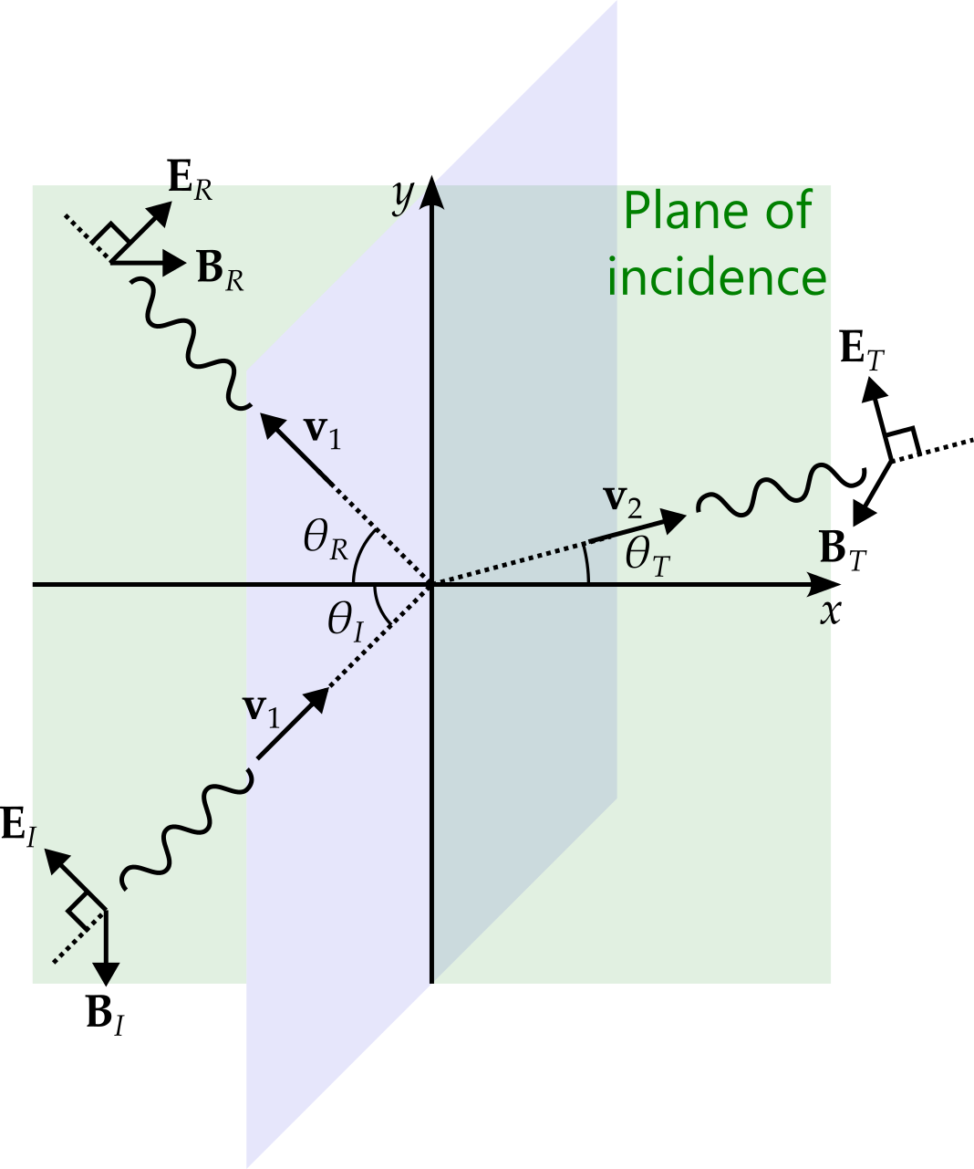
4.3.4 Oblique incidence (part 2)

When the incident light is polarised perpendicular to the place of incidence, we find that the two remaining Fresnel equations are \[ E^0_R = \left(\frac{1 - \alpha\beta}{1 + \alpha\beta}\right)E^0_I, \qquad E^0_T = \left(\frac{2}{1 + \alpha\beta}\right)E^0_I. \] Showing that this is the case is left as an exercise.

Exercise

Show that for polarisation perpendicular to the plane of incidence, Fresnel’s equations are given by \[ E^0_R = \left(\frac{1 - \alpha\beta}{1 + \alpha\beta}\right)E^0_I, \qquad E^0_T = \left(\frac{2}{1 + \alpha\beta}\right)E^0_I. \] Figure 4.4 may be of help.

Figure 4.4: The incident wave striking obliquely, with polarisation perpendicular to the plane of incidence. The illustrated electric field is pointing out of the page in all three cases, while the magnetic field lies in the plane of incidence.