7 Four-vectors
While we have managed without them thus far, the concept of a 4-vector is a powerful one in special relativity and absolutely vital in general relativity. They can be useful in both simplifying calculations and clarifying concepts. We will start, however, by taking a closer look at vectors in three dimensions first, noting the various ways in which vectors are defined. Then we introduce 4-vectors and also index notation and the Einstein summation convention, which may be of use in future courses.
7.1 Setting \(c = 1\)
For the rest of these notes, we will assume that we are using units in which \(c = 1\) and we will remove all the \(c\)’s from our equations. Hence, the Lorentz transformation becomes \[ \begin{aligned} t &= \gamma\left(t' + vx'\right),\\ x &= \gamma\left(x' + vt'\right),\\ y &= y',\\ z &= z', \end{aligned} \] where \[ \gamma = \frac{1}{\sqrt{1 - v^2}}, \] while the velocity addition formula becomes \[ v = \frac{v_1 + v_2}{1 + v_1v_2} \] and the formula for energy becomes simply \(E = \gamma m\).
This should simplify some of our calculations. If we really need to get a final result in terms of standard SI units, we can always reinsert factors of \(c\) in our final result to get a value in the desired units.1
1 If you perform dimensional analysis on our equations in their new form, you will find distances being added to durations, energies equal to masses and all sorts of atrocities. Do not worry! Use dimensional analysis to work out where the \(c\)’s should go after you have obtained your result.
7.2 Vectors — a review
It is possible that you are familiar with various definitions of a vector, or alternatively you might simply feel that you know a vector when you see one. It will be useful to review and distinguish between some of the definitions you may have seen, before introducing 4-vectors.
7.2.1 Row and column vectors
It is likely that the first types of vectors that you encountered were either row or column vectors, e.g. \[ \begin{pmatrix} 4.0\\ 6.2\\ -2.1 \end{pmatrix} , \qquad \begin{pmatrix} 2.0 & -1.1 & -2.9 \end{pmatrix} \] The numbers contained might be the components of the velocity of a particle in three dimensions, or could be the balances of the bank accounts of three people.2
2 The latter example does not seem very ‘physical’ when compared with quantities such as velocity, force, etc. We will see that it also differs in its transformation properties later.
Given a physical quantity such as velocity as a column vector, the values of the numbers mean little unless one is also provided with details of the coordinate system being used. The column vector as written above is merely shorthand for \[ 4.0\mathbf{i} + 6.2\mathbf{j} - 2.1\mathbf{k}, \] so to know which direction the vector points in, we need to know where the basis vectors \(\mathbf{i}\), \(\mathbf{j}\), \(\mathbf{k}\) point, or equivalently, the direction of the \(x\), \(y\) and \(z\) axes.
7.2.2 Abstract vectors
More recently, you should have seen a more abstract definition of a vector as an element of a vector space3. Vectors may be added, e.g. \(\mathbf{u} + \mathbf{b}\), multiplied by a number4, e.g. \(4\mathbf{u}\), and the operations of addition and multiplication must obey a collection of rules (or axioms)5, e.g. \[ a(\mathbf{u} + \mathbf{v}) = a\mathbf{u} + a\mathbf{v}. \] Additional structure, e.g. inner products, might (or might not) also be added on top of the basic vector space structure.
3 The study of vector spaces is called linear algebra.
4 Often referred to as a scalar.
5 We will not provide all the axioms here.
A wide range of mathematical objects qualify as vectors in this sense. In quantum mechanics you will see wave functions, \(\phi(\mathbf{x})\), treated as vectors and will have already seen quantum states written as vectors using Dirac notation, e.g. \(\left(\ket{\phi} + \ket{\psi}\right)/\sqrt{2}\).
7.2.3 Physical vectors
An intuitive notion of a physical6 vector is that it is an object with both magnitude and direction. This, however, is a little vague, so let’s attempt to clarify by considering how two different observers might view a vector.
6 I find it tempting to think of the abstract definition as the mathematician’s definition of a vector and this more physical approach as leading to the physicist’s definition. However, physicists really ought to know both definitions, so I will stick to ‘abstract’ and ‘physical’, for want of better adjectives.
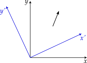
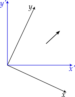
Figures 7.1 and 7.2 illustrate how, when viewed from a rotated frame of reference, the vector is rotated in the opposite direction. While the vector remains the same, the numbers used to represent it, i.e. its components, are different in each frame of reference, related via the application of a rotation matrix.
We now define a vector to be an object that transforms, under rotations7, in the same way as the displacement vector. The physical quantities that you know to be vectors, e.g. velocity, force, angular momentum, the gradient of a scalar field, all transform correctly. The bank balances of three people, mentioned earlier, do not and so, according to this definition, do not form a vector.
7 If we also insist that a vector must transform like a displacement vector under reflections then we find that quantities such as angular momentum do not transform in quite the right way. (Try it and see.) These are referred to as pseudovectors or axial vectors while quantities like the velocity are true vectors.
7.3 Defining 4-vectors
Having reminded ourselves of the properties and definitions of vectors, we now define 4-vectors.
Definition 7.1 (4-vectors) A 4-tuplet, \(A = (A_0, A_1, A_2, A_3)\) is called a 4-vector8 if it transforms in the same way as the displacement \((\delta t, \delta x, \delta y, \delta z)\) under a Lorentz transformation. That is, we require that \[ \begin{aligned} A_0 &= \gamma\left(A_0' + vA_1'\right),\\ A_1 &= \gamma\left(A_1' + vA_0'\right),\\ A_2 &= A_2',\\ A_3 &= A_3' \end{aligned} \] under a Lorentz transformation in the \(x\)-direction, and similar for Lorentz transformations in the \(y\) and \(z\) directions.9
8 It doesn’t really matter whether we write this as a column or a row vector.
9 \(A_0\) is referred to as the time component. The spatial components, \(A_1\), \(A_2\) and \(A_3\) should also transform correctly under rotations, so as to form a vector in three dimensions.
7.4 Properties of 4-vectors
4-vectors are useful because of their properties and in particular, because observers in different frames will always agree on the inner product of two 4-vectors, given a suitable definition of the inner product. Some of these properties are listed below.
7.4.1 Linearity
If \(A\) and \(B\) are both 4-vectors, then so are \(\lambda A + \mu B\).10 This follows directly from the linearity of the Lorentz transformation. If this is not readily apparent, you should do the next exercise.
10 We would certainly hope that this is the case, since otherwise the 4-vectors would not form a vector space!
Assuming that both \(A\) and \(B\) are 4-vectors, confirm that if we Lorentz transform \(A\) and \(B\) then the components of \(\lambda A + \mu B\) transform in the same way.
7.4.2 Invariance of the norm
We have already shown for the displacement vector that \[ (\delta t)^2 - (\delta x)^2 - (\delta y)^2 - (\delta z)^2 \] is unchanged under a Lorentz transformation, i.e. \[ (\delta t)^2 - (\delta x)^2 - (\delta y)^2 - (\delta z)^2 = (\delta t')^2 - (\delta x')^2 - (\delta y')^2 - (\delta z')^2. \] Since any 4-vector transforms like \((\delta t, \delta x, \delta y, \delta z)\), it must be the case that \[ A_0^2 - A_1^2 - A_2^2 - A_3^2 = A_0^2 - \left|\mathbf{A}\right|^2 \] is also Lorentz invariant. This quantity is the square of the norm and this property is analogous to the way in which the norm (i.e. length) of an ordinary 3-vector is not affected by rotations.
7.4.3 Invariance of inner products
We can define the inner product of two 4-vectors, \(A\) and \(B\), to be \[ A.B = A_0B_0 - A_1B_1 - A_2B_2 - A_3B_3 = A_0B_0 - \mathbf{A}.\mathbf{B}. \] Now consider performing a Lorentz transformation in the \(x\) direction. Since \(A_2\), \(A_3\), \(B_2\) and \(B_3\) are unchanged, we will focus on the zeroth and first components. \[ \begin{aligned} A_0B_0 - A_1B_1 &= \gamma^2(A_0' + vA_1')(B_0' + vB_1') - \gamma^2(A_1' + vA_0')(B_1' + vB_0')\\ &= \gamma^2(A_0'B_0' + \cancel{vA_1'B_0'} + \bcancel{vA_0'B_1'} + v^2A_1'B_1'\\ &\qquad\qquad\qquad - A_1'B_1' - \bcancel{vA_0'B_1'} - \cancel{vA_1'B_0'} - v^2A_0'B_0')\\ &= \frac{1}{1 - v^2}\left((1 - v^2)A_0'B_0' + (v^2 - 1)A_1'B_1')\right)\\ &= A_0'B_0' - A_1'B_1'. \end{aligned} \] Hence the inner product is the same in both frames.
It is this ability to construct Lorentz invariant quantities from 4-vectors that makes them so useful.
7.5 Examples of 4-vectors
Let’s start with something that is not a 4-vector. Consider the derivative of a displacement with respect to time, i.e. \[ \left(\frac{dt}{dt}, \frac{dx}{dt}, \frac{dy}{dt}, \frac{dz}{dt}\right). \] This is not a 4-vector. While \((dt, dx, dy, dz)\) transforms correctly, the denominator \(dt\) is also changed by a Lorentz transformation and this spoils the transformation of the whole.
We can, however, differentiate with respect to the proper time, \(\tau\), since this is independent of the frame. Hence \[ V = \left(\frac{dt}{d\tau}, \frac{dx}{d\tau}, \frac{dy}{d\tau}, \frac{dz}{d\tau}\right) = \left(\gamma, \gamma\mathbf{v}\right) \] is a 4-vector known as the 4-velocity. Notice that the spatial components form the proper velocity that we briefly described earlier. Notice also that \[ V.V = \gamma^2 - \gamma^2v^2 = \gamma^2(1 - v^2) = 1. \]
Now multiply the 4-velocity by the mass of the particle, to get \[ P = \left(\gamma m, \gamma m\mathbf{v}\right) = \left(E, \mathbf{p}\right). \] Since the mass of a particle also does not depend on the frame, this is also a 4-vector called the energy-momentum 4-vector. We see that \[ P.P = m^2V.V = m^2, \] which is the relationship \(E^2 - p^2 = m^2\) that we discovered earlier.
We can, of course, continue to differentiate with respect to the proper time. Then \(dV/d\tau\) gives the acceleration 4-vector \(A\), while \(dP/d\tau\) gives the force vector \(F\).11
11 We even find that \(F = mA\) when considering 4-acceleration and 4-force, but note that the relationship between the acceleration 4-vector, \(A\), and the standard acceleration 3-vector is not a straightforward one.
7.6 Why the interest in 4-vectors?
So why are we interested in 4-vectors? Firstly, we find that certain physical quantities naturally combine to produce 4-vectors and, indeed, present difficulties when considered separately. Consider energy and momentum. You can tell me the energy of a particle in your frame of reference, but this is insufficient data for me to calculate the energy in my frame. Similarly, you can tell me the momentum of a particle in your frame and, again, this is insufficient for me to determine the momentum in my frame. If, however, you tell me the energy-mometum 4-vector in your frame, then a simple Lorentz transformation gives the energy-momentum in my frame. In this sense, energy and momentum are truly only parts of a unified object — the energy-momentum 4-vector.
An example we have not seen yet12 is that of the electric scalar potential, \(\phi\), and the magnetic vector potential, \(\mathbf{A}\). These too do not transform individually when changing frames, but transform as the electromagnetic 4-potential, \(\left(\phi, \mathbf{A}\right)\).13
12 But will see soon when you study electromagnetism.
13 This is part of the reason why we talk of a unified interaction, electromagnetism. Forces that are caused by a magnetic field in one frame of reference might be caused by an electric field in another, and vice versa.
14 It would also provide a way to tell inertial frames apart, breaking the principle of relativity.
15 Such an equation is described as being manifestly covariant, which just means that both sides clearly (or manifestly) transform in the same way under a change of frame. Such equations may also involve scalars — i.e. Lorentz invariant quantities such as the mass of a particle or the invariant interval — and objects known as tensors, which can be thought of as being built from 4-vectors. These objects all transform in such a way as to work together well, e.g. a tensor applied to a 4-vector produces another 4-vector. (If you try to build quantum mechanics in a Lorentz invariant manner, then other options, e.g. spinors become available. However, you are unlikely to need these for some time.)
A second reason to be interested in 4-vectors is that physical laws, buiding on the foundation of special relativity, are frequently written in terms of them. Suppose we have a proposal for a physical law, but where the two sides of the equation transform differently upon a change of frame. While such a law might hold in your frame of reference, it is unlikely to hold in any other frame. As such, it is not a particularly useful law14. If, however, your proposed law is written as an equation where both sides are 4-vectors, then if the law holds in your frame, it holds in any15.
7.7 A simple collision
We will now get some practice at using 4-vectors, in particular the energy-momentum 4-vector, by looking at a simple collision.
A particle of mass \(m\) and energy \(E\) collides elastically16 with an identical but stationary particle. Both particles then proceed at an angle of \(\theta\) with respect to the direction of the incident particle. How does this angle depend upon the initial conditions.
16 Energy is always conserved in special relativity. We define an elastic collision to be one where the masses of the particles do not change.
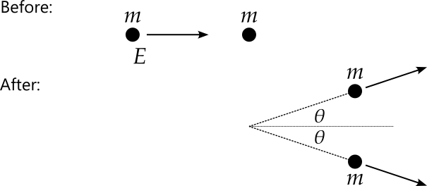
Writing the 4-momenta17 before and after the collision, we have18 \[ P_1 = (E, p, 0, 0), \qquad P_2 = (m, 0, 0, 0), \] and \[ \hat{P}_1 = \left(\hat{E}_1, \hat{p}_1\cos\theta, \hat{p}_1\sin\theta, 0\right), \quad \hat{P}_2 = \left(\hat{E}_2, \hat{p}_2\cos\theta, -\hat{p}_2\sin\theta, 0\right). \] We now apply conservation of 4-momentum, considering each component in term. Considering the third components, we see that before the collision the total momentum is zero in this direction, while afterwards, we have \(\hat{p}_1\sin\theta - \hat{p}_2\sin\theta\), so we get \(\hat{p}_1 = \hat{p}_2\). We can use this result to also show that \(\hat{E}_1 = \hat{E}_2\), since we know that \[ \hat{P}_1.\hat{P}_1 = \hat{E}_1^2 - \hat{p}_1^2 = m^2 \] and \[ \hat{P}_2.\hat{P}_2 = \hat{E}_2^2 - \hat{p}_2^2 = m^2. \] Hence we can rewrite the outgoing 4-momenta as \[ \hat{P}_1 = \left(\hat{E}, \hat{p}\cos\theta, \hat{p}\sin\theta, 0\right), \quad \hat{P}_2 = \left(\hat{E}, \hat{p}\cos\theta, -\hat{p}\sin\theta, 0\right). \]
17 4-momentum is just a shorter name for the energy-momentum 4-vector.
18 Here we will use subscripts to indicate the identity of the particle.
Now looking at the first two components, we get \[ \hat{E} = \frac{1}{2}\left(E + m\right) \] and \[ \hat{p} = \frac{p}{2\cos\theta}, \] so the outgoing momenta are now \[ \hat{P}_1 = \left(\frac{1}{2}\left(E + m\right), \frac{p}{2}, \frac{1}{2}p\tan\theta, 0\right), \quad \hat{P}_2 = \left(\frac{1}{2}\left(E + m\right), \frac{p}{2}, -\frac{1}{2}p\tan\theta, 0\right). \] We have now run out of conservation laws to apply, but we can still use \(\hat{P}_1.\hat{P}_1 = m^2\) to get \[ \frac{(E + m)^2}{4} - \frac{1}{4}p^2\left(1 + \tan^2\theta\right) = m^2. \] Noting that \(1 + \tan^2\theta = 1 / \cos^2\theta\) and rearranging now give \[ \cos^2\theta = \frac{E^2 - m^2}{E^2 + 2Em - 3m^2} = \frac{E + m}{E + 3m}. \]
This has solved the problem, but as usual we should check the classical limit. As any snooker player knows, in the classical limit the outgoing particles move at right angles to each other, so we should have \(\theta = \pi/4\) and \(\cos^2\theta = 1 / 2\). Checking our formula, in the classical limit we have \(E \simeq m\) and so \(\cos^2\theta \simeq 2m/4m = 1/2\) as required. If we also consider the relativistic limit when \(E \gg m\) then we find that \(\cos^2\theta \simeq 1\) and the two outgoing particles each move (almost) directly forward at an angle of \(\theta \simeq 0\).
7.8 Index notation and the Einstein summation convention
7.8.1 Index notation
If in future you continue to study physics that builds upon special relativity, e.g. by taking units in general relativity or in quantum fields and particles, then you will undoubtedly use both index notation for 4-vectors and the Einstein summation convention. This section introduces both of these ideas to prepare you, at least a little, for your future studies19.
19 My aim, therefore, is to enable you to use the notation, rather than to teach the abstract mathematics behind it or the technical terminology. However, you will notice from some of the sidenotes that I have not been able to entirely resist providing a little extra (non-examinable) material.
20 Does this not run the risk of confusing 4-vector index notation with raising a quantity to a power? Surprisingly, once you have some experience with this notation, you will find that the meaning of a superscript is usually clear from the context. However, when the notation is new to you, some confusion is possible. Why use superscripts instead of subscripts? Well, actually we use both, as you will soon see.
21 Now it looks like I am being deliberately confusing, using \(x\) for both the 4-vector and for its second component. Yes, I could have used \(X\) for the 4-vector, with components \(X^0\), \(X^1\), \(X^2\) and \(X^3\). However, in my experience, \(x\) is used more often than \(X\) for the position 4-vector. Moreover, we seldom write a 4-vector \(x\) without an index attached, which should reduce any confusion.
22 This is obvious here, but less so for other 4-vectors. Hence the time component of the energy-momentum 4-vector is the energy, while the momentum forms the spatial components.
You should already be familiar with index notation for ordinary 3-vectors, where a subscript is used to indicate a particular component of a vector. Index notation for 4-vectors is similar, except that for the examples we have seen thus far, a superscript20 is used instead. Hence, if we use \(x\) to represent the position of an event21 in spacetime then we have \[ x^0 = t, \quad x^1 = x, \quad x^2 = y, \quad x^3 = z. \] The zeroth component \(x^0\) is referred to as the time component, while the others are the spatial components22.
We commonly use Greek letters for indices, e.g. \(x^{\mu}\). While, technically speaking this represents a single component of the 4-vector, depending on the value of \(\mu\), we often use \(x^\mu\) as shorthand for the whole 4-vector, i.e. \[ x^\mu = (x^0, x^1, x^2, x^3) = (t, x, y, z). \]
If we use a subscript23 on a 4-vector then the spatial components24 are multiplied by -1, i.e. \[ x_\mu = (x_0, x_1, x_2, x_3) = (x^0, -x^1, -x^2, -x^3) = (t, -x, -y, -z). \] Notice that we can now write the inner product of the 4-vector, \(x^\mu\), with itself as \[ \sum_{\mu = 0}^3 x_\mu x^\mu = t^2 - x^2 - y^2 - z^2, \] which you should notice as the invariant interval. If we have two 4-vectors, \(A^\mu\) and \(B^\mu\), then the inner product between them is \[ \begin{aligned} \sum_{\mu = 0}^3 A_\mu B^\mu &= A_0B^0 + A_1B^1 + A_2B^2 + A_3B^3\\ &= A^0B^0 - A^1B^1 - A^2B^2 - A^3B^3, \end{aligned} \] which matches our earlier definition.
23 Mathematically, 4-vectors with subscripts are covectors, or dual vectors. 4-vectors with superscripts are sometimes referred to as contravariant, with those with subscripts being covariant.
24 Much like for the invariant interval, the signs here depend on the convention being used. If we use \[ s^2 = -t^2 + x^2 + y^2 + z^2, \] i.e. the `mostly positive’ convention for the invariant interval instead, then we would multiply only the time component by -1 when lowering the index.
7.8.2 Einstein summation convention
While writing a single summation sign is not too taxing but more complex calculations can easily include many summations. To eliminate the need to write summation signs for each of these, it is useful to use the Einstein summation convention. This convention states that if an index, e.g. \(\mu\), is repeated as both a superscript (‘up’) and subscript (‘down’), then we sum over this index. Our previous sum for the inner product may now be written as simply \(A_\mu B^\mu\), with the summation implied. In other words \[ A_\mu B^\mu := \sum_{\mu = 0}^3 A_\mu B^\mu. \]
7.8.3 The metric tensor
Let \(g_{\mu\nu}\) be the metric25 tensor26, represented by the matrix \[ \begin{pmatrix} 1 & 0 & 0 & 0\\ 0 & -1 & 0 & 0\\ 0 & 0 & -1 & 0\\ 0 & 0 & 0 & -1 \end{pmatrix}. \] Multiplying a 4-vector, with a superscript index, by the metric tensor has the effect of lowering the index. That is, given 4-vector \(A^\mu\), we have \(A_\mu = g_{\mu\nu}A^\nu\). For example, writing this using matrix notation for the position 4-vector, we have \[ \begin{pmatrix} t\\ -x\\ -y\\ -z \end{pmatrix} = \begin{pmatrix} 1 & 0 & 0 & 0\\ 0 & -1 & 0 & 0\\ 0 & 0 & -1 & 0\\ 0 & 0 & 0 & -1 \end{pmatrix} \begin{pmatrix} t\\ x\\ y\\ z \end{pmatrix}. \]
25 To a mathematician, a metric space is a set of points together with a function, called a metric, for giving the distance between a pair of points. This metric must satisfy a set of axioms one would expect a distance to satisfy. Given that we are studying special relativity, here the metric gives the invariant interval, rather than a standard distance.
26 Think of a tensor as being a matrix, but like 4-vectors, a tensor must have the correct transformation properties. In particular, the result of multiplying a 4-vector by a tensor should be another 4-vector (though perhaps with index ‘down’).
27 An index appearing three times, e.g. \(g_{\mu\mu}A^\mu\) is bad news!
Notice how the indices behave in the equation \(A_\mu = g_{\mu\nu}A^\nu\). Any unmatched indices — in this case \(\mu\) — must match on each side of the equation. Repeated indices are known as dummy indices. Since they are summed over, it matters little which label we use for them. That is, \(g_{\mu\nu}A^\nu\) is the same as \(g_{\mu\rho}A^\rho\) which is the same as \(g_{\mu\sigma}A^\sigma\). Therefore, in calculations it may be beneficial to rename a dummy index, in order to avoid clashing with the label for another index.27
Notice that this now means that we can write the inner product of 4-vectors \(A^\mu\) and \(B^\mu\) as \(A^\mu g_{\mu\nu} B^\nu\).
We also define \(g^{\mu\nu}\) to be the inverse of the metric tensor28. That is \[ g^{\mu\nu}g_{\nu\rho} = \delta^\mu_\rho, \] where \(\delta^\mu_\rho\) is the identity matrix29. It is then a simple matter to see that \(g^{\mu\nu}\) raises indices, for \[ g^{\mu\nu}A_\nu = g^{\mu\nu}g_{\nu\rho}A^\rho = \delta^\mu_\rho A^\rho = A^\mu. \]
28 Of course, numerically this is the same matrix. Note though that if you study general relativity in the future then the metric may take a much more complicated form and no longer be its own inverse.
29 Ignoring the placement of the indices, you may also recognise this as the Kronecker delta, with elements equal to one if \(\mu = \rho\) and zero otherwise.
7.8.4 The Lorentz transformation
We may now write the Lorentz transformation as a matrix30, \({\Lambda^\mu}_\nu\). For the transformation in the \(x\)-direction, this is \[ {\Lambda^\mu}_\nu = \begin{pmatrix} \gamma & -\beta\gamma & 0 & 0\\ -\beta\gamma & \gamma & 0 & 0\\ 0 & 0 & 1 & 0\\ 0 & 0 & 0 & 1 \end{pmatrix} \] and we see that for a 4-vector, \(A^\mu\), we have31 \(A'^\mu = {\Lambda^\mu}_\nu A^\nu\), i.e. \[ \begin{pmatrix} A'^0\\ A'^1\\ A'^2\\ A'^3 \end{pmatrix} = \begin{pmatrix} \gamma & -\beta\gamma & 0 & 0\\ -\beta\gamma & \gamma & 0 & 0\\ 0 & 0 & 1 & 0\\ 0 & 0 & 0 & 1 \end{pmatrix} \begin{pmatrix} A^0\\ A^1\\ A^2\\ A^3 \end{pmatrix}. \] ::: {.callout-note title=“Exercise” collapse=false} Perform the matrix multiplication above and compare with previous equations for the Lorentz transformation. :::
30 Note that this time, this is not a tensor. A tensor usually represents something physical whose representation is transformed as we change reference frame. The Lorentz transformation, on the other hand, is the matrix we use to perform this change of frame.
31 In his book, “A First Course in General Relativity”, Bernard Schutz uses an interesting alternative notation, where the annotation (prime, dash, hat, bar, etc.) is applied to the index. In other words, \(A^{\mu'} = {\Lambda^\mu}_\nu A^\nu\) or \(A^{\bar{\mu}} = {\Lambda^\mu}_\nu A^\nu\). While I like this approach, since it emphasises that \(A\) is the same vector throughout and that it is the coordinate system that is changing, I will use the more commonly seen approach of annotating the 4-vector \(A\) in the main text.
Given matrix \({A^\mu}_\nu\), find a simple, short way to write its trace.
Using the Einstein summation convention, the trace is simply \({A^\mu}_\mu\), since this will sum over the elements \({A^0}_0\), \({A^1}_1\), \({A^2}_2\) and \({A^3}_3\), as required.
7.8.5 Derivatives
Using this index notation, we write \(\frac{\partial}{\partial x^\mu}\) as simply \(\partial_\mu\). If \(\phi\) is a scalar field then \[ \partial_\mu\phi = \left(\frac{\partial\phi}{\partial t}, \frac{\partial\phi}{\partial x}, \frac{\partial\phi}{\partial y}, \frac{\partial\phi}{\partial z}\right) \] which you should recognise as a four-dimensional version of the gradient32 of \(\phi\). Similarly, if we have a 4-vector field, \(A^\mu\), then \[ \partial_\mu A^\mu = \frac{\partial A^0}{\partial x^0} + \frac{\partial A^1}{\partial x^1} + \frac{\partial A^2}{\partial x^2} + \frac{\partial A^3}{\partial x^3}, \] which is a four-dimensional version of the divergence. We may also consider the object \(\partial_\mu A^\nu\).
32 If you have not yet seen the gradient of a scalar field or the divergence of a vector field, you will soon do so when you learn vector calculus. Note that the index notation used here can be used in three dimensions just as well as four, in which case \(\partial_\mu\phi\) and \(\partial_\mu A^\mu\) are different notations for \(\nabla\phi\) and \(\nabla.\mathbf{A}\).
7.8.6 Example: Proving that the inner product, \(a^\mu g_{\mu\nu}b^{\nu}\), is Lorentz invariant
After a Lorentz contraction, \(a^\mu\) becomes \(a'^\mu = {\Lambda^\mu}_\nu a^\mu\) and \(b^\mu\) becomes \(b'^\mu = {\Lambda^\mu}_\nu b^\mu\). Being careful to avoid too many copies of the same index, we find that \[ \begin{aligned} a'^\mu g_{\mu\nu}b'^\nu &= {\Lambda^\mu}_\rho a^\rho g_{\mu\nu}{\Lambda^\nu}_\sigma b^\sigma\\ &= a^\rho{(\Lambda^T)_\rho}^\mu g_{\mu\nu}{\Lambda^\nu}_\sigma b^\sigma\\ &= a^\mu{(\Lambda^T)_\mu}^\rho g_{\rho\sigma}{\Lambda^\sigma}_\nu b^\nu. \end{aligned} \] To understand the second line, first note that the expression in the first line is just a collection of numbers (components) being multiplied together, with a few (implicit) summation signs in front. We are therefore free to reorder the items that are being multiplied. Furthermore, recall that taking the transpose of a matrix is equivalent to switching the order of the indices. So while the ‘up’ index remains ‘up’ and the ‘down’ index remains ‘down’, taking the transpose means that the \(\rho\) now comes before the \(\mu\). Finally note that the indices are now arranged so that this looks like matrix multiplication33 — we will exploit this fact in a bit. In the third line, seeing that all of the indices are dummy indices, we use the freedom to rename them.
33 Recall that given matrix \(A\) and vector \(x\), we have \[ \left(Ax\right)_i = \sum_{j}A_{ij}x_j, \] while if \(B\) is also a matrix then \[ \left(AB\right)_{ij} = \sum_{k}A_{ik}B_{kj}. \] That is, the indices being summed over are adjacent.
We now notice that if \[ g_{\mu\nu} = {(\Lambda^T)_\mu}^\rho g_{\rho\sigma}{\Lambda^\sigma}_\nu \] then \(a^\mu g_{\mu\nu}b^{\nu}\) will be invariant for any vectors \(a^\mu\) and \(b^\mu\). Well, let’s see. \[ \begin{aligned} {(\Lambda^T)_\mu}^\rho g_{\rho\sigma}{\Lambda^\sigma}_\nu &= \begin{pmatrix} \gamma & -\beta\gamma & 0 & 0\\ -\beta\gamma & \gamma & 0 & 0\\ 0 & 0 & 1 & 0\\ 0 & 0 & 0 & 1 \end{pmatrix} \begin{pmatrix} 1 & 0 & 0 & 0\\ 0 & -1 & 0 & 0\\ 0 & 0 & -1 & 0\\ 0 & 0 & 0 & -1 \end{pmatrix} \begin{pmatrix} \gamma & -\beta\gamma & 0 & 0\\ -\beta\gamma & \gamma & 0 & 0\\ 0 & 0 & 1 & 0\\ 0 & 0 & 0 & 1 \end{pmatrix} \\ &= \begin{pmatrix} 1 & 0 & 0 & 0\\ 0 & -1 & 0 & 0\\ 0 & 0 & -1 & 0\\ 0 & 0 & 0 & -1 \end{pmatrix} = g_{\mu\nu}. \end{aligned} \] This confirms the Lorentz invariance of the inner product.