5  The structure of spacetime

Before the advent of special relativity, we could believe in the notion that space and time were separate entities. Putting to one side inaccuracies in our timekeeping, the duration of time between two events was something that everyone could agree on. Furthermore, while different observers might use different \(x\), \(y\) and \(z\) coordinates and might not agree on \(\delta x\) if they were facing in different directions, distances and lengths could be agreed upon.

After special relativity, the distinction is less clear. Observers may disagree on both durations and distances. Furthermore, the Lorentz contraction mixes together time and spatial coordinates in a manner similar to that in which a rotation about the \(z\)-axis mixes \(x\) and \(y\) coordinates. While it was always possible to consider time to be a fourth dimension, to add to the three dimensions of space, it is tempting now to consider the resulting 4-dimensional spacetime more seriously.

We will start by considering the invariant interval — something all observers can agree on and which looks much like a distance, but one which ties together the time and spatial dimensions. We will then consider a method for visualising spacetime — the Minkowksi diagram.

5.1 The invariant interval

Given two events, and letting \(\delta t\), \(\delta x\), \(\delta y\) and \(\delta z\) be the separation between the events in each of the 4 dimensions, consider the quantity¹ \[ (\delta s)^2 = c^2(\delta t)^2 - (\delta x)^2 - (\delta y)^2 - (\delta z)^2. \] This is called the invariant interval².We will claim that this is Lorentz invariant, i.e. that observers in any inertial frame³ will agree on the value for \((\delta s)^2\).

¹ There are two conventions for the signs here. The one used here (mostly negative) tends to be used those studying quantum field theory and particle physics. The alternative, where the first term has a minus sign and the others do not (mostly positive) tends to be preferred by relativists. (If you want to study quantum field theory in curved spacetime, get used to both!)

² Some authors call \(\delta s\) the invariant interval. Others call \((\delta s)^2\) the invariant interval. Of course, it really doesn’t matter — they are both invariant.

³ I have used \(\delta t\), \(\delta x\), etc., instead of just \(t\) and \(x\), to ensure that observers in translated frames of reference (i.e. stationary with respect to one another but offset by some distance) also agree. You may wish to confirm that observers will agree on \((\delta s)^2\), even if their frames are translated or rotated with respect to each other, or moving relative to each other in any direction.

We will confirm this for frames moving relative to each other along the \(x\)-axis, using the Lorentz transformation. Since this does not affect the \(y\) and \(z\) coordinates, we will ignore these for now. (For convenience, we will also drop the \(\delta\)’s, just to keep the calculation tidier.) We find that \[ \begin{aligned} c^2\delta t^2 - x^2 &= \frac{c^2\left(t' + vx'/c^2\right)^2 - \left(x' + vt'\right)}{1 - v^2 / c^2}\\ &= \frac{t'^2\left(c^2 - v^2\right) - x'^2\left(1 - v^2 / c^2\right)}{1 - v^2 / c^2}\\ &= c^2t'^2 - x'^2 \end{aligned} \] and hence \((\delta s)^2 = (\delta s')^2\).

The invariant interval looks much like a distance (squared)⁴, with the only problem being the minus signs. It is related to Lorentz transformations in much the same way as distance is related to rotations. That is, the interval is Lorentz invariant, whereas a distance is rotation invariant.

⁴ And would have looked even more like a distance if I had chosen the ‘mostly positive’ convention.

5.2 Separation

You will have noticed that, in contrast to a squared distance, \((\delta s)^2\) may take any value. The sign of \((\delta s)^2\) reveals how pairs of events may be causally related in different ways. That is, it tells us whether one event could possibly affect the other.

Before we discuss the three ways in which events may be separated, it will be useful to let \(d\) be the spatial separation of the two events, i.e. \[ d = \sqrt{(\delta x)^2 + (\delta y)^2 + (\delta z)^2}. \]

Timelike separation: If \((\delta s)^2 > 0\) then the two events are timelike separated. We find that \(c\left|\delta t\right| > d\) and hence there is time to travel from one event to the other. Now imagine an observer who does this, at a constant velocity. Then in her frame of reference, both events happen at the same location.

If events are timelike separated, then the quantity \(\delta s / c\) is called the proper time between them, and is denoted as \(\delta \tau\) or just \(\tau\). It is the time that elapses for an inertial⁵ observer travelling between the two events.

⁵ Actually, the term ‘proper time’ is also used for non-inertial observers. The proper time along a timelike worldline (see later) is defined as the time measured by a clock following that line. This depends not only on the two events but on the worldline taken — recall the twin paradox. However, if I discuss proper time without mentioning a worldline, assume that I mean the proper time for an inertial traveller.

⁶ The word ‘proper’ here does not mean ‘correct’. It comes from the French ‘propre’ meaning ‘own’, as in a clocks own time, or an objects own length. In other words, the length of the object in the objects frame of reference.

Spacelike separation: If \((\delta s)^2 < 0\) then the two events are spacelike separated. We find that \(c\left|\delta t\right| < d\) and hence it is impossible for even light to travel from either event to the other. In this case, there is a frame in which the two events happen simultaneously. In this frame, we find that \(d = \left|\delta s\right|\) and so \(\left|\delta s\right|\) is called the proper distance or proper length⁶.

Exercise

Consider two spacelike separated events with \(\delta y = \delta z = 0\) in frame \(F\). Find a frame, \(F'\), in which the two events are simultaneous, and the relative velocity of the frames.

Solution

Two events are separated by \(\delta t\) and \(\delta x\) in frame \(F\). We require a frame, \(F'\), such that \(\delta t' = 0\). Using the Lorentz transformation \[ \delta t' = \gamma\left(\delta t - v\delta x/c^2\right), \] we see that we require \[ \delta t - v\delta x/c^2 = 0 \] and hence \[ v = \frac{c^2\delta t}{\delta x}. \]

Lightlike separation: If \((\delta s)^2 = 0\) then the two events are lightlike separated. Since \(c\left|\delta t\right| = d\), only light can get from one event to the other. It is not possible to find a frame where the events are simultaneous or happen in the same place.⁷

⁷ But it a photon can travel from one event to another, can we not choose its frame, within which each event would be at the same location? Alas, no. Now that we are studying special relatively, frames cannot travel at the speed of light. But why not? Ask yourself two questions. How fast does the photon move in its frame? How fast must a photon move in any frame?

5.3 Minkowski diagrams

In considering space and time conjoined into a four dimensional spacetime, we may also consider how we might visualise this construct through the use of diagrams. Alas, four dimensional paper and computer screens have not been invented yet, but if the action all takes place in one spatial dimension, the other two may be suppressed so that we plot time against the spatial coordinate \(x\). Consider figure 5.1.

Figure 5.1: A spacetime diagram, illustrating the arrival of a train at a station, the boarding of a passenger and the departure of the train. An observer remains stationary on the platform.

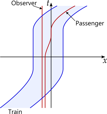
Here we see a train arriving at a station, a passenger boarding and the train leaving. An observer waits with the passenger on the platform until the train arrives, but remains stationary throughout.⁸

⁸ You might be more used to plotting graphs where \(t\) is on the horizontal axis. However, in relativity, the convention is for the time axis to point upwards on spacetime diagrams, so you will need to get used to this.

The red and blue lines here are the worldlines of two people and of the rear and front of the train.

Exercise

Suppose that figure 5.1 shows a realistic train, i.e. one that can travel no more than 300km/h. On this diagram, what would the worldline of a photon look like?

Solution

A photon’s worldline would be indistinguishable from a horizontal line on this figure. If, for example, the units on the \(x\)-axis were metres and those on the time axis were seconds, then a photon’s worldline would have a gradient of \(1 / 3\times10^8 \simeq 3\times10^{-9}\).

In special relativity, dealing with faster objects means that it makes sense to rescale the axes so that a greater expanse of space can be accommodated. If the axes are scaled such that the worldlines of photons lie at 45 degrees to the time axis, e.g. by plotting \(ct\) against \(x\) or by choosing units where \(c = 1\), then the result is a Minkowski diagram.

Figure 5.2: A Minkowski diagram.

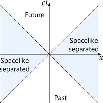
If we consider the centre of the diagram to represent here and now, then events in the shaded regions of figure 5.2 are spacelike separated from us. It is neither possible for us to have any impact on these events, or for these events to affect the here and now, since in either case this would require something to travel faster than the speed of light. Things happening here and now can have an impact in the region labelled ‘future’, while the causes of events happening here and now must lie in the region labelled ‘past’.⁹

⁹ This description of the possible causal relationships between events is referred to as the causal structure of spacetime.

¹⁰ Where here we require that the origin of frames must be colocated when \(t = t' = 0\).

You might now argue that surely any event on the diagram with a positive \(ct\) coordinate is in the future of the origin event, whether we at the origin can affect the event or not. The issue here is that observers in a different frame might ascribe a negative \(ct'\) value for the same event. By this logic, such an event would be in the future in one frame and the past in the other. It is better, therefore, to say that whether such an event is in the future or past is indeterminate, or to simply say that such events are spacelike separated from us. In contrast, those events in the region labelled ‘future’ have a positive \(ct\) coordinate in all frames¹⁰.

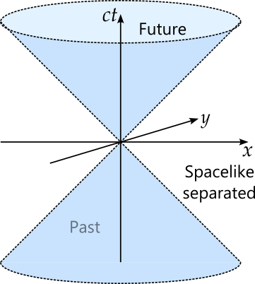
The dashed lines in figure 5.2 are referred to as the light cone. The reason for the name becomes apparent when we reintroduce a second spatial coordinate.

Figure 5.3: A light cone.

5.4 The Lorentz transformation visualised

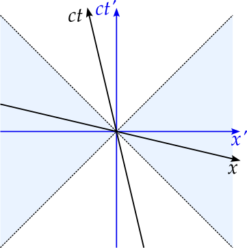
Ignoring the \(y\) and \(z\) coordinates, we may rewrite the Lorentz transformation and its inverse as \[ \begin{aligned} ct &= \gamma(ct' + vx' / c),\\ x &= \gamma(x' + vct' / c) \end{aligned} \] and \[ \begin{aligned} ct' &= \gamma(ct - vx / c),\\ x' &= \gamma(x - vct / c).\\ \end{aligned} \] Now suppose that we have a Minkowski diagram with axes \(x\) and \(ct\) and we wish to superimpose the \(x'\) and \(ct'\) axes. We need only set \(ct'=0\) and \(x'=0\) respectively. We get \[ \begin{aligned} ct' = 0 \quad &\Rightarrow \quad ct = \frac{v}{c}x = \beta x,\\ x' = 0 \quad &\Rightarrow \quad x = \frac{v}{c}ct = \beta ct. \end{aligned} \] Hence the \(x'\) axis is at a gradient of \(\beta\) while the \(ct'\) axis has a gradient of \(1 / \beta\), as shown in figure 5.4.

Figure 5.4: The Lorentz transformation visualised using a Minkowski diagram.

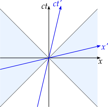
Notice how events between the \(x\) and \(x'\) axes have positive time coordinates in one frame and negative time coordinates in the other, illustrating how it would be problematic to label such events as being in the future or the past.

We can, of course, start by drawing the Minkowski diagram in \(x'\) and \(ct'\) coordinates and then superimpose the \(x\) and \(ct\) axes instead, producing figure 5.5.

Figure 5.5: Plotting the \(x\) and \(ct\) axes on the \(x'\) – \(ct'\) Minkowski diagram.

To find out where any tick marks on the axes move to, we need only take the points \((x', ct') = (1, 0)\) and \((x', ct') = (0, 1)\) and use the transform to find the \(x\) and \(ct\) coordinates we find that they are \((x, ct) = (\gamma, \beta\gamma)\) and \((x, ct) = (\beta\gamma, \gamma)\).

5.5 Rapidity

The rapidity, \(\phi\) is defined by \[ \tanh\phi = \beta = \frac{v}{c}. \] It increases when \(v\) increases, decreases when \(v\) decreases and so is essentially another notion of the speed of the particle. Why should we want to know about rapidity, when we already have the speed?

It can be easier to discuss the rapidities of particles. Describing two particles as having rapidities of 5 and 10 is clearer than stating that their speeds are \(0.999999775c\) and \(0.9999999959c\).¹¹ Here, however, we will emphasise that using rapidity can produce some elegant results and allow us to reframe the Lorentz transformation so that it begins to look like a more familiar transformation — a rotation.

¹¹ Though it might be more intuitive still to discuss the energy of the particles instead.

¹² You can find this formula in the appendix on hyperbolic functions.

¹³ This is provided we are only working in one spatial dimension.

Consider a particle moving in the \(x\) direction at speed \(v_1\) in a frame that moves at \(v_2\) in the same direction with respect to us. We are interested in calculating the velocity, \(v\), of the particle in our frame. Of course, we already know how to do this — we can use the velocity addition formula. We let \(\beta_1 = v_1 / c\), \(\beta_1 = \tanh\phi_1\) and similarly define \(\beta_2\), \(\phi_2\), \(\beta\) and \(\phi\). Using the velocity addition formula, we have \[ \tanh\phi = \beta = \frac{\beta_1 + \beta_2}{1 + \beta_1\beta_2} = \frac{\tanh\phi_1 + \tanh\phi_2}{1 + \tanh\phi_1\phi_2}. \] You would be forgiven at this point for not recognising the addition formula for the hyperbolic tangent¹² But if we do recognise the formula, we can continue \[ \tanh\phi = \beta = \frac{\beta_1 + \beta_2}{1 + \beta_1\beta_2} = \frac{\tanh\phi_1 + \tanh\phi_2}{1 + \tanh\phi_1\phi_2} = \tanh(\phi_1 + \phi_2) \] and we see that \(\phi = \phi_1 + \phi_2\). We see that the rapidities combine in a much simpler way than the velocities¹³. Moreover, there is also no upper limit on the rapidity — as particles approach the speed of light, their rapidities increase towards infinity.

The Lorentz transformation can also be rewritten in terms of the rapidity, in which case we find that it takes a particularly pleasing and vaguely familiar form. Start by writing the Lorentz transformation in terms of \(ct\) and \(x\): \[ \begin{aligned} ct &= \gamma(ct' + vx' / c) = \gamma(ct' + \beta x'),\\ x &= \gamma(x' + vct' / c) = \gamma(x' + \beta ct'). \end{aligned} \] Now write \(\gamma\) and \(\beta\gamma\) in terms of the rapidity. We have \[ \gamma = \frac{1}{\sqrt{1 - \beta^2}} = \frac{1}{\sqrt{1 - \tanh^2\phi}} = \cosh\phi, \] while \[ \beta\gamma = \tanh\phi\cosh\phi = \sinh\phi. \] If we now write the Lorentz transformation in matrix form, we get \[ \begin{pmatrix} ct\\ x \end{pmatrix} = \begin{pmatrix} \cosh\phi & \sinh\phi\\ \sinh\phi & \cosh\phi \end{pmatrix} \begin{pmatrix} ct'\\ x' \end{pmatrix} . \] This should look almost like a rotation. The trigonometric functions have been replaced with hyperbolic functions and there is a missing minus sign, but there is a definite similarity.

Remark 5.1 (Time as an imaginary distance (optional)). We can make the Lorentz transformation look even more rotation-like¹⁴. We might imagine a duration of time to be like an imaginary distance and define \(\tau = ict\). The Lorentz transformation becomes \[ \begin{pmatrix} \tau\\ x \end{pmatrix} = \begin{pmatrix} \cosh\phi & i\sinh\phi\\ -i\sinh\phi & \cosh\phi \end{pmatrix} \begin{pmatrix} \tau'\\ x' \end{pmatrix} . \] which we can write using ordinary trigonometric functions as \[ \begin{pmatrix} \tau\\ x \end{pmatrix} = \begin{pmatrix} \cos i\phi & -\sin i\phi\\ \sin i\phi & \cos i\phi \end{pmatrix} \begin{pmatrix} \tau'\\ x' \end{pmatrix} . \] This would appear to finally be a rotation, but by an imaginary angle — the rapidity times \(i\).

¹⁴ Here we are straying a little from the main content of the course to look at something that perhaps should be considered as a mathematical curiosity.

It is also worth noting that (minus) the interval, \(-s^2\), when written in these new coordinates, becomes \[ -s^2 = \tau^2 + x^2 + y^2 + z^2 \] and hence the interval looks like an ordinary distance squared.

While the above is more of a curiosity, Lorentz transformations and rotations can be compared in another way. We may define a rotation, in three dimensions, to be a linear transformation that preserves distances \[ s^2 = x^2 + y^2 + z^2 \] (and orientation), while a Lorentz transformation is a linear transformation that preserves the interval \[ s^2 = c^2t^2 - x^2 - y^2 - z^2. \]