Cauchy principal value integrals
A pole on the contour
If a contour of integration goes around an isolated singularity, the residue of the singularity contributes to the value of the integral. If an isolated singularity lies outside the contour, then it simply does not contribute. But what if a (non-removable) singularity lies on the contour?
Your likely first reaction is technically correct — if a pole lies on the contour, then we cannot calculate the integral. It is best to avoid this situation if possible, by arranging for the contour to avoid singularities. However, we might wish to calculate a real integral from minus infinity to infinity, but where the integrand has an unavoidable pole on the real axis. While technically this integral does not exist, this might not keep us from wanting to find its value!
A motivational example
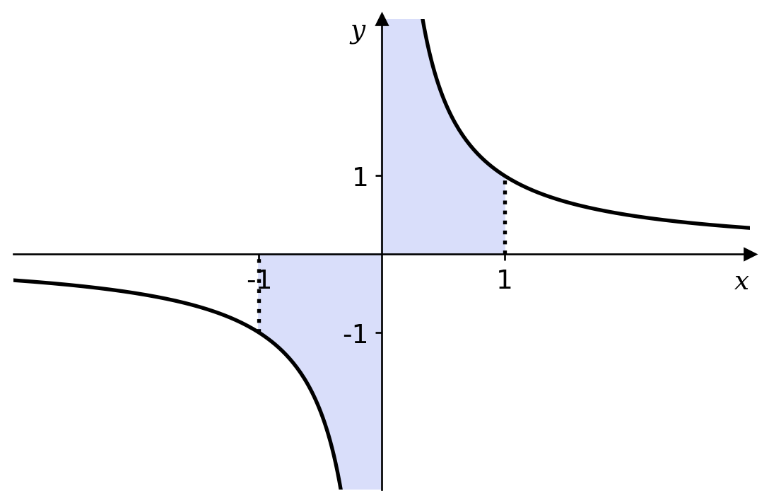
We wish to calculate \[ \int_{-1}^1\frac{1}{x}\,dx. \] Technically, this integral does not exist, but figure 1 suggests a value anyway.
Here the shaded area to the right is clearly equal to that on the left and, since the integral is the difference between these two areas, the integral must be zero — right? Wrong. An improper integral such as this one is defined to be \[ \int_{-1}^1 \frac{1}{x}\,dx = \lim_{\delta \rightarrow 0}\int_{-1}^{-\delta} \frac{1}{x}\,dx + \lim_{\epsilon \rightarrow 0}\int_{\epsilon}^{1} \frac{1}{x}\,dx \] and neither of these limits exist — both areas are infinite1.
1 So, the idea of subtracting one shaded area from the other is reasonable. The problem is that we get \(\infty - \infty\), which is undefined.
The Cauchy principal value
If we really want this integral to have a value (and this value to be zero) then there is a way. We can use the Cauchy principal value of the integral, defined to be \[ \mathcal{P}\int_{-1}^1 \frac{1}{x}\,dx = \lim_{\epsilon \rightarrow 0}\left[\int_{-1}^{-\epsilon} \frac{1}{x}\,dx + \int_\epsilon^1 \frac{1}{x}\,dx\right] = 0 \] For both the improper integral and the principal value, we integrate up to a short distance of the singularity and take a limit. The important differences between this and the improper integral is that here we approach the singularity symmetrically and the limit is take after the integrals are summed.
More generally, if \(a < b < c\) and \(f(x)\) has a singularity at \(x = b\), then \[ \mathcal{P}\int_a^c f(x)\,dx = \lim_{\epsilon \rightarrow 0}\left[\int_a^{b - \epsilon} f(x)\,dx + \int_{b + \epsilon}^c f(x)\,dx\right] = 0 \]
Exercise
What happens if we approach the singularity at \(x = 0\) asymmetrically? Calculate \[ \lim_{\epsilon \rightarrow 0}\left[\int_{-1}^{-2\epsilon} \frac{1}{x}\,dx + \int_\epsilon^1 \frac{1}{x}\,dx\right]. \]
Solution
\[ \begin{aligned} \lim_{\epsilon \rightarrow 0}\left[\int_{-1}^{-2\epsilon} \frac{1}{x}\,dx + \int_\epsilon^1 \frac{1}{x}\,dx\right] &= \lim_{\epsilon \rightarrow 0}\left[(\log(2\epsilon) - \log1) + (\log1 - \log\epsilon)\right]\\ &= \log 2 \neq 0. \end{aligned} \] By approaching the singularity asymmetrically in other ways, we can make the value of the integral equal to any real number we choose!
Cauchy principal values and contour integration
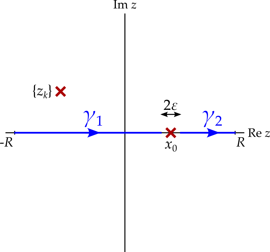
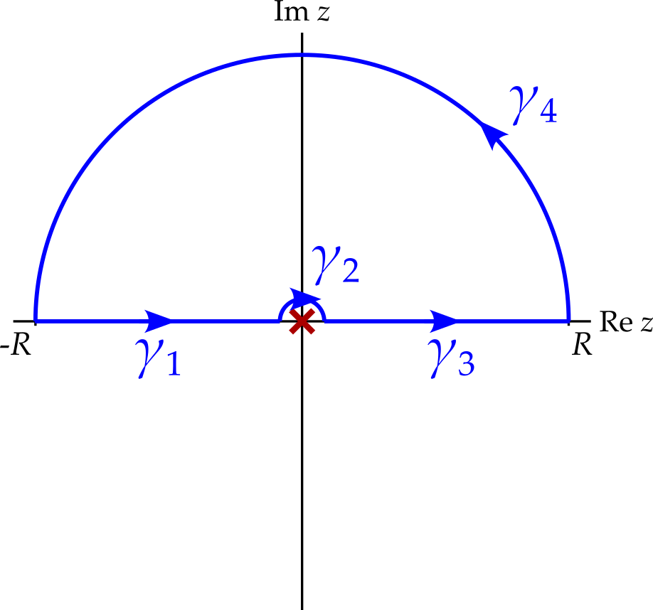
Now suppose that we have an integral \[ \int_{-\infty}^\infty f(x)\,dx, \] where function \(f\) has a simple pole at \(x = x_0\), and we wish to use complex analysis to find the Cauchy principal value, \[ I = \mathcal{P}\int_{-\infty}^\infty f(x)\,dx = \lim_{\epsilon \rightarrow 0}\left[\int_{-\infty}^{x_0 - \epsilon} f(x)\,dx + \int_{x_0 + \epsilon}^\infty f(x)\,dx\right] \] At this stage, the contour consists of two disconnected parts as shown in figure 2.
As in chapter 9 , if the integrand approaches zero fast enough as \(\left|z\right| \rightarrow \infty\) in the upper half-plane then we may add a semicircular arc there, of radius \(R\), knowing that the integral along this arc will approach zero as \(R \rightarrow \infty\). However, this is not enough to close the contour — we must also join \(x_0 - \epsilon\) to \(x_0 + \epsilon\), while avoiding the singularity. This can be done in two ways: with a semicircle below \(x_0\) or a semicircle above. For now, we choose to close the contour below the singularity as shown in figure 3.
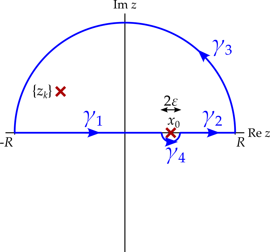
Knowing that the integral along \(\gamma_3\) approaches zero, calculating the integral we want (that along \(\gamma_1\) and \(\gamma_2\)) now consists of the following two steps.
- Calculate the integral around the entire contour using the residue theorem
- Subtract the integral along \(\gamma_4\).
So what value does the integral along \(\gamma_4\) approach as the radius, \(\epsilon\) approaches zero? Since \(x_0\) is a simple pole, we can write that \[ f(z) = \frac{a_{-1}}{z - x_0} + g(z), \] where \(g\) is holomorphic at and in a neighbourhood of \(x_0\). In particular, \(g(z)\) is bounded in this neighbourhood while, as \(\epsilon\) approaches zero, so does the length of the contour. Hence \[ \lim_{\epsilon \rightarrow 0}\int_{\gamma_4}g(z)\,dz = 0. \] Meanwhile, writing the path as \(\gamma_4(\theta) = x_0 + \epsilon e^{i\theta}\), for \(\pi < \theta < 2\pi\), we get \[ \begin{aligned} \int_{\gamma_4}\frac{a_{-1}}{z - x_0}\,dz &= a_{-1}\int_\pi^{2\pi}\frac{1}{\epsilon e^{i\theta}}i\epsilon e^{i\theta}\,d\theta\\ &= \pi ia_{-1}. \end{aligned} \] Hence \[ \lim_{\epsilon \rightarrow 0}\int_{\gamma_4}f(z)\,dz = \pi ia_{-1}, \] which is precisely half what we would get if \(\gamma_4\) encircled \(x_0\) completely.
Using the residue theorem, the integral around the entire contour, \(\gamma = \gamma_1 + \gamma_4 + \gamma_2 + \gamma_3\) is \[ \oint_{\gamma} f(z)\,dz = \sum_k 2\pi i\operatorname{Res}\left[f\right]_{z_k} + 2\pi ia_{-1}, \] where \(z_k\) indicates the location of any other singularities in the upper half plane. So \[ \begin{aligned} I &= \sum_k 2\pi i\operatorname{Res}\left[f\right]_{z_k} + 2\pi ia_{-1} - \pi ia_{-1}\\ &= \sum_k 2\pi i\operatorname{Res}\left[f\right]_{z_k} + \pi ia_{-1}\\ &= \sum_k 2\pi i\operatorname{Res}\left[f\right]_{z_k} + \pi i\operatorname{Res}\left[f\right]_{x_0}. \end{aligned} \]
Exercise
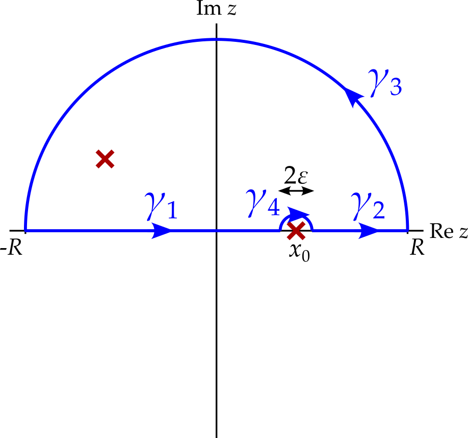
Examine what happens if the contour had been completed by going above the singularity at \(x_0\)
Solution
If the contour had gone above the singularity instead then we would have found that \[ \oint_{\gamma} f(z)\,dz = \sum_k 2\pi i\operatorname{Res}\left[f\right]_{z_k}, \] since the singularity at \(x_0\) would no longer be inside the contour. Meanwhile, contour \(\gamma_4\) would go clockwise halfway around the singularity, so \[ \begin{aligned} \lim_{\epsilon \rightarrow 0}\int_{\gamma_4} f(z)\,dz &= \int_{\gamma_4}\frac{a_{-1}}{z - x_0}\,dz\\ &= a_{-1}\int_\pi^{0}\frac{1}{\epsilon e^{i\theta}}i\epsilon e^{i\theta}\,d\theta\\ &= -\pi ia_{-1}. \end{aligned} \] Substracting this from the integral around the whole contour, we get \[ \begin{aligned} I &= \sum_k 2\pi i\operatorname{Res}\left[f\right]_{z_k} + \pi ia_{-1}\\ &= \sum_k 2\pi i\operatorname{Res}\left[f\right]_{z_k} + \pi i\operatorname{Res}\left[f\right]_{x_0} \end{aligned}, \] i.e. the same result as before.
Example 1 Let us calculate \[ \int_{-\infty}^\infty \frac{\sin x}{x}\,dx. \] Notice that while the integrand has a singularity at \(x = 0\), this is a removable singularity. We could simply define the integrand to be equal to 1 when \(x = 0\). However, it is not clear how we would close the contour.
We notice that \[ \frac{\sin x}{x} = \operatorname{Im}\frac{e^{ix}}{x} \] and notice that it would be nice if we could write \[ \int_{-\infty}^\infty \frac{\sin x}{x}\,dx = \operatorname{Im}\int_{-\infty}^\infty \frac{e^{ix}}{x}\,dx, \] since then we could use Jordan’s lemma, closing the contour in the upper half plane. Unfortunately, the removable singularity at \(x = 0\) is removable no longer — \(e^{ix} / x\) has a simple pole there. However, we can write \[ \int_{-\infty}^\infty \frac{\sin x}{x}\,dx = \operatorname{Im}\mathcal{P}\int_{-\infty}^\infty \frac{e^{ix}}{x}\,dx, \]
We therefore analytically continue, replacing \(x\) with \(z\), and close the contour as show in figure 5.
Using Jordan’s lemma, the integral along \(\gamma_4\) approaches zero as \(R \rightarrow \infty\). The integral around the entire contour is zero, since there are no singularities inside. The integral along \(\gamma_2\) approaches \(-\pi i\operatorname{Res}\left[e^{iz} / z\right] = -\pi i\). Therefore, \[ \mathcal{P}\int_{-\infty}^\infty \frac{e^{ix}}{x}\,dx = \int_{\gamma_1}\frac{e^{iz}}{z}\,dx + \int_{\gamma_3}\frac{e^{iz}}{z}\,dx = \pi i. \] We have therefore determined that \[ \int_{-\infty}^\infty \frac{\sin x}{x}\,dx = \pi. \]