5  Multivalued functions and branches

5.1 Real multivalued functions

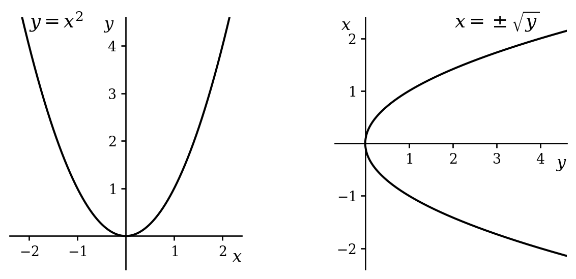
Before thinking about multivalued functions in complex analysis, it is worth noting that you have undoubtedly considered the possibility of multivalued real functions already. We often encounter functions that are ‘many-to-one’¹ and may wish to find the inverse² of such a function, in order, perhaps, to find solutions to \(x^2 = 4\) or \(\sin \theta = 0.5\). Figures 5.1 and 5.2 shows what we would like to do.

¹ To use more technical language, functions that are not injections.

² See below for why I wince slightly as I write this!

Figure 5.1: We consider inverting the many-to-one function \(f(x) = x^2\), illustrated on the left, producing the multivalued square root ‘function’ shown on the right.

So, what is the inverse of, for example, the function \(f(x) = x^2\). We will see that the technically correct answer is that it does not have an inverse. However, if we could allow a function to take multiple values, then we could say that the inverse is \(f^{-1}(x) = \pm\sqrt{x}\).

Figure 5.2: Graph of the function \(f(x) = x^2\) and its ‘inverse’ \(f(y) = \pm\sqrt{y}\).

5.1.1 Being fussy

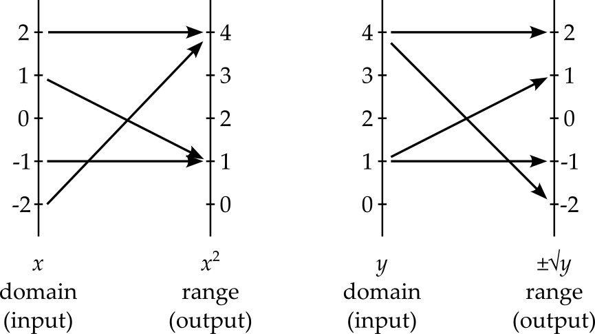
Alas, mathematicians are fussy regarding what is and is not a function. In particular, for every input, \(x\), to a function, there must be a unique output, \(f(x)\). Our ‘inverse’ function, \(f^{-1}(x) = \pm\sqrt{x}\), therefore fails to be a function.

There are advantages to insisting that functions be single valued. For example, when some writes \(\sqrt{4}\), we know that the value being referred to is \(+2\), not \(-2\). Things can get complicated quickly if we combine multiple multivalued functions together. Also, defining concepts such as differentiation becomes challenging if, for each value of \(x\), the function being differentiated can take multiple different values.

So how do we fix our function \(f^{-1}(x) = \pm\sqrt{x}\)? Well, we first ensure that the domain of the function is just the non-negative reals, to ensure that each input has at least one output. We then select only the positive number that, when squared, gives \(x\), i.e. the principal value. We are left with the standard definition of \(\sqrt{x}\).³ There is little downside here - the square root function is continuous and differentiable (i.e. well-behaved) and the only risk is that a student might think that \(y^2 = x\) means that \(y = \sqrt{x}\).

³ It should be emphasised at this point that the square root function is not the inverse of \(f(x) = x^2\). Technically, a function can only have an inverse if it is a bijection, that is a function that is one-to-one and onto.

Figure 5.3: Two well-behaved, single-valued square root functions. \(f(x) = +\sqrt{x}\) is the standard definition, but \(f(x) = -\sqrt{x}\) is equally well behaved, being both continuous and differentiable.

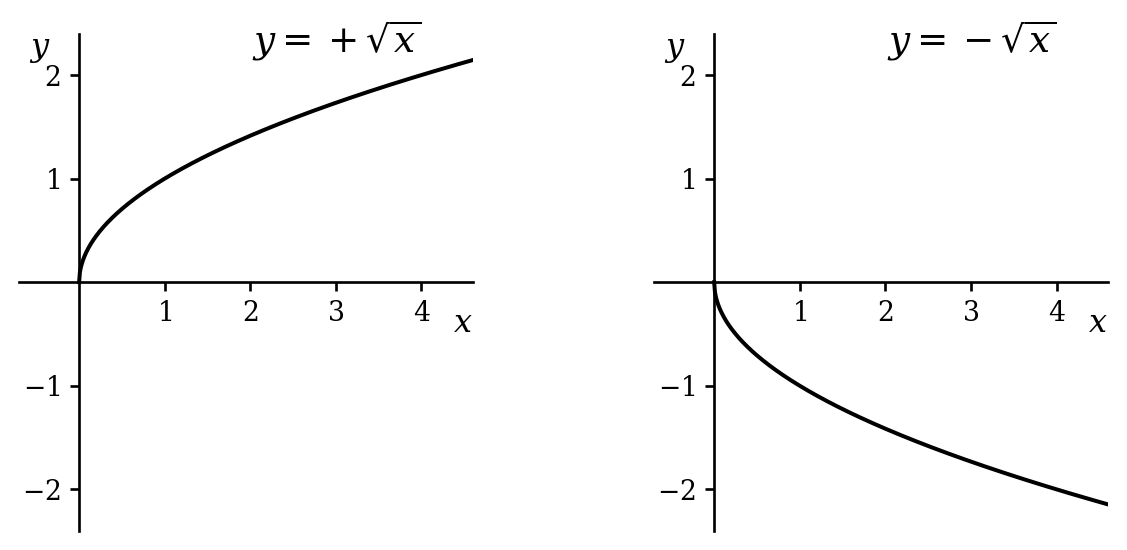
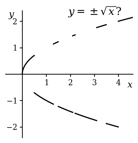
Notice that we could have chosen the negative square roots and produced an equally well behaved function. However, it would have been unwise to choose the positive square root for some values of \(x\) and the negative square root for others - the resulting function would inevitably have discontinuites and fail to be differentiable.

Figure 5.4: An unwise way to define a single-valued square root function. While this function is single-valued and squaring it will return \(x\), the function behaves poorly, with numerous discontinuities.

How do we avoid making a poor choice when turning a multivalued function into a single-valued one? We have been looking at a simple case, but in future we may wish to look at more complicated multivalued functions and we certainly will want to be able to handle complex functions. One strategy is to fix a single value of the function, e.g. \(x^{1/2} = 1\) when \(x = 1\). Then we slowly change \(x\) and ask ourselves, which value should we choose for \(x^{1/2}\) as \(x\) changes so as to maintain continuity? In this case, it should be clear that we will always need to choose the positive square root. And so, starting from \(x = 1\), our definition of \(x^{1/2}\) is extended along the positive real line.

5.2 The complex square root

Let us continue to look at the square root function, but extend our analysis to the complex plane. Naturally, the function \(f(z) = z^2\) continues to be many-to-one. If \(z^2 = re^{i\theta}\) then there are two possible values for \(z\), since \[ z = \sqrt{r}e^{i\theta / 2} \quad \Rightarrow \quad z^2 = re^{i\theta} \] and \[ z = -\sqrt{r}e^{i\theta / 2} \quad \Rightarrow z^2 = re^{i\theta}. \] Hence, \(z^{1/2}\) must be multivalued. To turn it into a proper function, we need to make it single valued. How should we do this? Unlike in the real case, there is not an obvious, best choice. Consider \(z = -i\). Should we choose \((-i)^{1/2} = e^{3\pi i/4} = (-1 + i)/\sqrt{2}\) or \((-i)^{1/2} = e^{-\pi i/4} = (1 + -i)/\sqrt{2}\)?

Our aim will be to produce a single-valued function, \(z^{1/2}\) that is

• consistent with the real function \(f(x) = \sqrt{x}\) and
• is as well-behaved as possible, i.e. continuous and holomorphic.

Alas⁴, unlike in the real case, we will have to tolerate some disappointment - we will not be able to make the function well-behaved everywhere.

⁴ Spoiler alert

5.2.1 Analytic continuation

Our strategy for ensuring that we produce a well-behaved single-valued function will mirror that mentioned at the end of section 5.1.1. We will start by requiring \(z^{1/2}\) to take positive values on the positive real axis, i.e. to agree with \(f(x) = \sqrt{x}\). We will then slowly increase the argument, \(\theta\), of \(z\), choosing values for \(z^{1/2}\) that ensure continuity with those values fixed before. As \(\theta\) increases⁵, we sweep the complex plane, eventually choosing values for \(z^{1/2}\) for all \(z\)

⁵ In what follows, we will always use \(\theta\) to refer to \(\arg z\) and \(r\) to refer to \(\left|z\right|\).

⁶ In what follows, it might be useful to focus on moving around a single path, e.g. the unit circle, by considering only \(r = 1\).

So⁶, starting from \(\theta = 0\), where we have already decided to set \(z^{1/2} = \sqrt{r}\), we slowly increase \(\theta\) to some small positive value \(\epsilon\) and we reach \(z = re^{i\epsilon}\). There are two options for the value of \(z^{1/2}\): \[ z^{1/2} = \sqrt{r}e^{i\epsilon / 2} \approx \sqrt{r} \qquad \text{and} \qquad z^{1/2} = -\sqrt{r}e^{i\epsilon / 2} \approx -\sqrt{r}. \] Since we have only moved a tiny distance in the complex plane, the value of \(z^{1/2}\) should be very close to \(\sqrt{r}\). If it were instead close to \(-\sqrt{r}\) then this would imply a discontinuity in the function, which we wish to avoid. Hence we must choose \[ z^{1/2} = \sqrt{r}e^{i\epsilon / 2}. \] We now continue to increase \(\theta\) to \(2\epsilon\). Again, we have two choices for the square root of \(z = re^{2i\epsilon}\), \[ z^{1/2} = \sqrt{r}e^{i\epsilon} \qquad \text{and} \qquad z^{1/2} = -\sqrt{r}e^{i\epsilon}. \] The first of these is close to the previous value of \(\sqrt{r}e^{i\epsilon / 2}\); the second is not. Hence, to avoid creating a discontinuity, we again must select the first option.

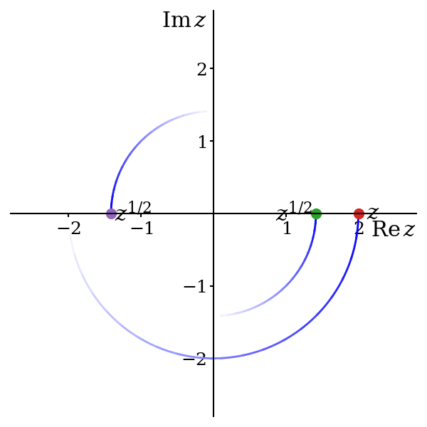
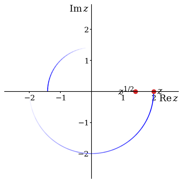
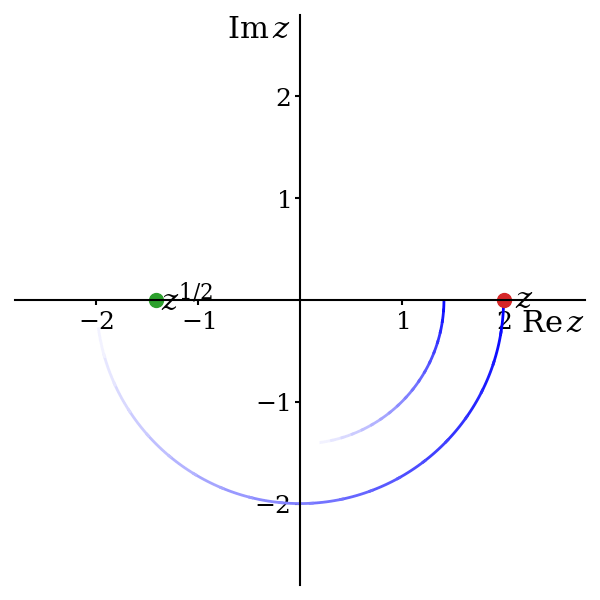
You should be able to see where this is going: we must always choose \(z^{1/2} = \sqrt{r}e^{i\theta / 2}\), since otherwise there must be a discontinuity where \(z^{1/2}\) jumps from \(\sqrt{r}e^{i\theta / 2}\) to \(-\sqrt{r}e^{i\theta / 2}\). So \(\theta\) increases and reaches \(\pi/2\) and we fix \(i^{1/2}\) to be \(e^{i\pi/4} = (1 + i) / \sqrt{2}\). It then reaches \(\pi\), and we fix \((-1)^{1/2} = e^{i\pi/2} = i\). Further still, as \(\theta\) reaches \(3\pi/2\), we fix \((-i)^{1/2}\) equal to \(e^{3\pi/4} = (-1 + i)/\sqrt{2}\). Finally, \(\theta\) reaches \(2\pi\) and we set \(1^{1/2} = e^{\pi i} = -1\).

Woah, hold on there! We require our function to be single valued and we already have \(1^{1/2} = 1\). So we leave out this final step, stopping once we have assigned a value for \(z^{1/2}\) to all \(z \in \mathbb{C}\). Yet we still have a problem. We have carefully ensured that \(z^{1/2}\) varies smoothly around the circle, but we find that we cannot avoid a discontinuity at the end⁷, with the value jumping from \(-1\) to \(1\) as we return to \(z = 1\).

⁷ One might make an analogy with the telephone game, where children sit in a circle and a message is whispered from one child to the next until it returns to the first child. In each step, the message undergoes only minor changes, but by the end of the game, the message may be completely different from how it started.

Figure 5.5: Evolution of the (single-valued) square root of \(z\) as \(z\) moves around the circle \(|z| = 2\). Notice how \(z\) moves smoothly around the circle, while \(z^{1/2}\), being a single-valued function, is forced to jump back to its original value once \(z\) returns to \(2\).

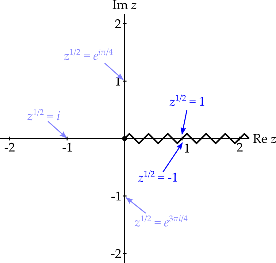
To recap, we have successfully created a single valued function \[ z^{1/2} = r^{1/2}e^{i\theta / 2},\qquad \text{for } 0 \leq \theta < 2\pi \] defined across the whole complex plane and holomorphic everywhere except at the discontinuity on the positive real axis. Notice the constraint on the values of \(\theta\) that we are permitting. As we cross the positive real axis from below, we force \(\theta\) to change, discontinuously, from \(2\pi\) to zero and this becomes the source of the discontinuity in \(z^{1/2}\).

5.3 Branch cuts

The discontinuity along the positive real axis is called a branch cut.

Figure 5.6: The function \(z^{1/2}\) with branch cut taken along the positive real axis. Crossing the real axis from below at \(z = 1\), the value of the function jumps from -1 to 1.

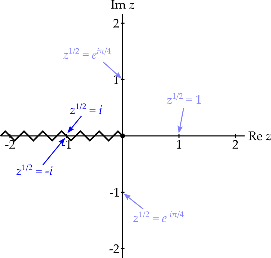
Notice that we could have produced a different single valued version of \(z^{1/2}\) by moving clockwise and anticlockwise from the positive real axis simultaneously, meeting at the negative real axis. This produces \[ z^{1/2} = r^{1/2}e^{i\theta / 2},\qquad \text{for } -\pi < \theta \leq \pi. \] The different range permitted for \(\theta\) in the formula results in the branch cut begin on the negative real axis. (This gives the principal values of \(z^{1/2}\) for all \(z\).)

Figure 5.7: The function \(z^{1/2}\) with branch cut taken along the negative real axis. Crossing the real axis from below at \(z = -1\), the value of the function jumps from \(-i\) to \(i\). Notice how the values of \(z^{1/2}\) at some points are different from those in figure 5.6.

As you can probably guess by now, there is considerable flexibility in where the branch cut is placed. For example, we could place it along the positive imaginary axis, or at 45 degrees to the positive real axis. Indeed, it need not even be a straight line, provided it starts at \(z = 0\) and goes to infinity without crossing itself.

5.4 Branches

Wherever we decide to place the branch cut, we find that the multifunction \(z^{1/2}\) has two branches. Suppose that the branch cut is placed along the positive real axis and that we define \[ z^{1/2} = r^{1/2}e^{i\theta / 2},\qquad \text{for } 0 \leq \theta < 2\pi. \tag{5.1}\] This is our first branch. The second branch, with the branch cut in the same location, is simply minus the first, i.e. \[ z^{1/2} = -r^{1/2}e^{i\theta / 2},\qquad \text{for } 0 \leq \theta < 2\pi. \tag{5.2}\]

5.5 Branch points

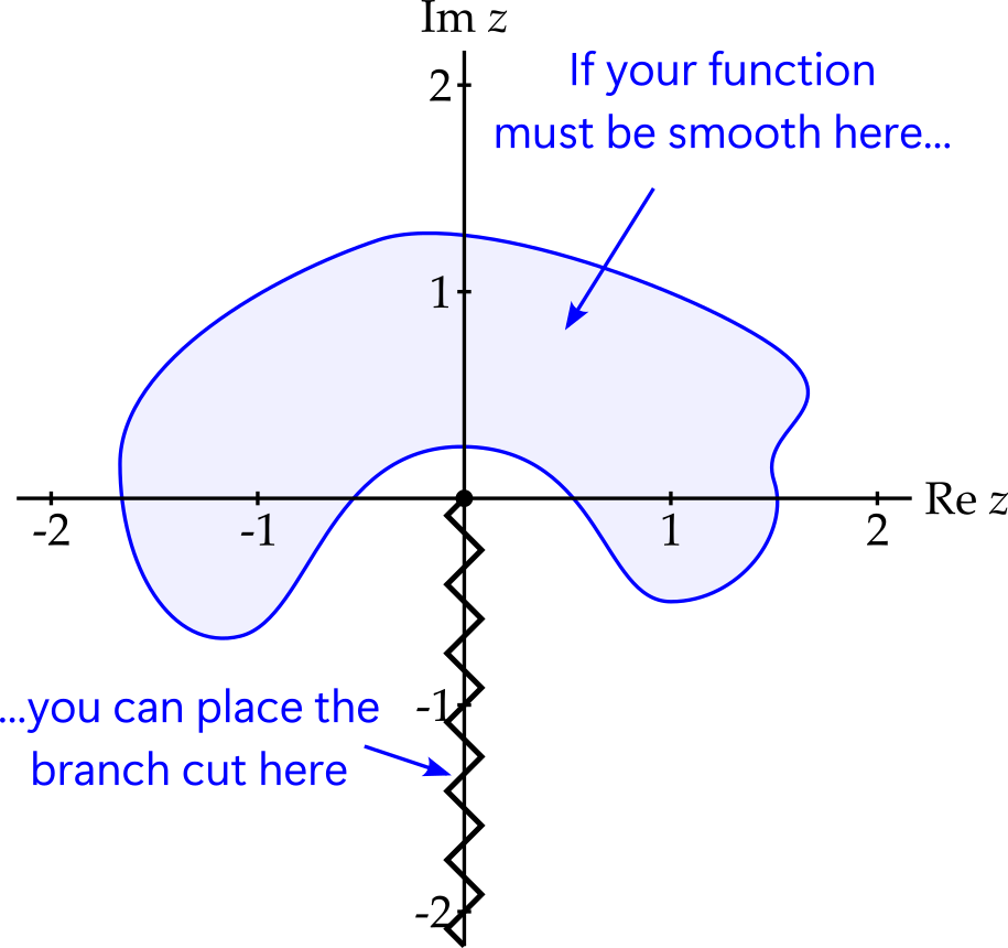
You may have noticed that, given a (simply connected⁸) region, one can create a version of \(z^{1/2}\) that is single valued and well-behaved in the region, provided the branch cut can be placed so as to avoid it. This is illustrated in figure 5.8.

⁸ No holes.

Figure 5.8: Ensuring that the function is continuous on a region by choosing a branch cut that avoids it.

However, if a region contains \(z = 0\) then \(z^{1/2}\) cannot be defined so as to be both single-valued and well-behaved. Traversing any loop that encloses \(z = 0\) and requiring \(z^{1/2}\) to vary smoothly causes \(z^{1/2}\) to return to minus its original value - an unavoidable discontinuity. The point \(z = 0\) is referred to as a branch point - no single-valued version of \(z^{1/2}\) can behave well there.

What if we permit a multivalued \(z^{1/2}\) and traverse a loop, e.g. the unit circle, around the branch point at \(z = 0\)? Starting at \(\theta = 0\), on the first time around the loop, the function takes the value \(e^{i\theta / 2}\), i.e. we are on the first branch of \(z^{1/2}\) (equation 5.1). Once we reach \(\theta = 2\pi\) and return to \(z = 1\), we find that, to continue to change \(z^{1/2}\) smoothly we must move on to the second branch (equation 5.2). Once we have gone around the loop twice, the multivalued \(z^{1/2}\) returns to its original value⁹.

⁹ Hence this version \(z^{1/2}\) may have the disadvantage of being multivalued - it is not technically a function - but the advantage of no need for a branch cut.

Figure 5.9: Evolution of the multivalued square root of \(z\) as \(z\) moves around the circle \(|z| = 2\). Notice that each \(z\) produces two values of \(z^{1/2}\): that visited on \(z\)s first lap around the origin (the first branch) and that visited on the second lap.

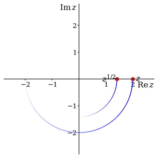
The order of a branch point is defined to be the number of times a path around it must be traversed in order for the multivalued function to return to its original value. Hence, for \(z^{1/2}\), \(z = 0\) is a branch point of order 2.

5.6 Further examples

Thus far we have focused on \(z^{1/2}\), but there are many other multivalued functions.

Example 5.1 The multivalued logarithm is defined as \[ \log z = \log\left(re^{i\theta + 2n\pi i}\right) = \log r + i(\theta + 2n\pi) \] If we restrict \(\theta\) to be within the interval \((-\pi, \pi]\) then the formula above defines an infinite number of branches of the function, one for each value of \(n\). Setting \(n = 0\) gives the principal value branch \[ \operatorname{Log}z = \log\left(re^{i\theta}\right) = \log r + i\theta, \qquad -\pi < \theta < \pi. \]

If we traverse any path that travels anticlockwise around the origin, starting on the negative real axis, then \(\theta\) increases from \(-\pi\) to \(\pi\) and \(\operatorname{Log}z\) increases by \(2\pi i\). Being single valued, it must then drop discontinuously to its original value before traversing the path again. We therefore have a branch cut on the negative real axis and a branch point at \(z = 0\).

Alternatively, if we consider the multifunction, \(\log z\), and want it to vary continuously, we might start on the \(n = 0\) branch, but after one trip anticlockwise around the origin we move up to the \(n = 1\) branch. A second trip anticlockwise then moves us up to the \(n = 2\) branch, and so on. Going clockwise results in us moving down the branches instead¹⁰.

¹⁰ Imagine a spiral staircase.

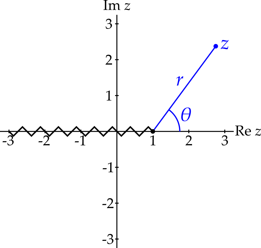
Example 5.2 Consider \(f(z) = (z - 1)^{1/3}\). Notice that this is \(w^{1/3}\) where \(w = z - 1\) and so in this case it is useful to write \(w = re^{i\theta}\) and hence \(z = 1 + re^{i\theta}\). Now \(w^{1/3}\) has three different values \[ \qquad r^{1/3}e^{i\theta / 3 - 2\pi i/3}, \qquad r^{1/3}e^{i\theta / 3}, \qquad r^{1/3}e^{i\theta / 3 + 2\pi i/3}, \] and the branch point is at \(w = 0\). Hence, in the \(z\)-plane, the branch point is at \(z = 1\)

Figure 5.10: Branch point and one choice for the branch cut of \((z - 1)^{1/3}\). Here we restrict the argument, \(\theta\), to be between \(-\pi\) and \(\pi\).

Now consider what happens to \(f(z)\) as \(z\) circles the branch point anticlockwise, starting from somewhere to the left of \(z = 1\) on the real axis. If we choose the first branch (defined as above with \(\theta \in (-\pi, \pi]\)), then upon completing the circle we reach the branch cut where this branch has a discontinuity. However, if we switch to the second branch as we cross the branch cut, then our value for \((z - 1)^{1/3}\) will change continuously as we cross the axis. After another cycle, we would need to switch to the third branch to maintain continuity. Finally, after one more cycle, we return to the first branch. Hence we have branch point of order 3 at \(z = 1\).

Example 5.3 Consider \(f(z) = (z^2 + 1)^{1/2}\). What do suitable branch cuts look like?

We rewrite \(f(z)\) as \[ f(z) = (z - i)^{1/2}(z + i)^{1/2}. \] We know that \(z^{1/2}\) has a branch point at \(z = 0\), so we expect \(z = i\) and \(z = -i\) to both be branch points of \(f(z)\). Let’s see if that is the case.

To help us with our analysis, we write \[ z - i = r_1e^{i\theta_1}, \qquad z + i = r_2e^{i\theta_2}. \]

Figure 5.11: Branch points for \((z^2 + 1)^{1/2}\) and some useful variables.

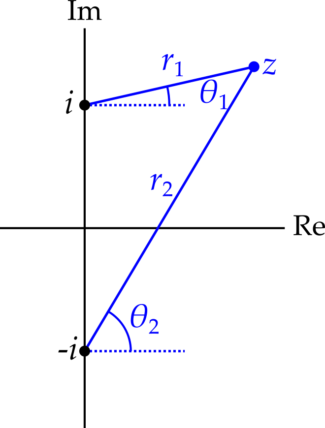
We may now write that \[ f(z) = \sqrt{r_1r_2}e^{i(\theta_1 + \theta_2)/2} \] Let’s investigate what happens to this function as we allow \(z\) to follow the four paths in the complex plane shown in figure 5.12.

Figure 5.12: Four paths.

The effect on f(z) of taking each of the four paths.

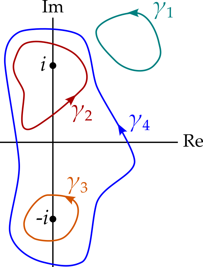
Path	Encloses	\(\theta_1\)	\(\theta_2\)	\(f(z)\)
\(\gamma_1\)	Neither	\(\theta_1 \rightarrow \theta_1\)	\(\theta_2 \rightarrow \theta_2\)	\(f(z) \rightarrow f(z)\)
\(\gamma_2\)	\(z = +i\)	\(\theta_1 \rightarrow \theta_1 + 2\pi\)	\(\theta_2 \rightarrow \theta_2\)	\(f(z) \rightarrow -f(z)\)
\(\gamma_3\)	\(z = -i\)	\(\theta_1 \rightarrow \theta_1\)	\(\theta_2 \rightarrow \theta_2 + 2\pi\)	\(f(z) \rightarrow -f(z)\)
\(\gamma_4\)	\(z = -i\) and \(+i\)	\(\theta_1 \rightarrow \theta_1 + 2\pi\)	\(\theta_2 \rightarrow \theta_2 + 2\pi\)	\(f(z) \rightarrow f(z)\)

Unsurprisingly, we see that if we take path \(\gamma_1\), which encircles neither branch point, then at the end of the cycle, \(f(z)\) returns to its orignal value.

However, if we take path \(\gamma_2\), circling only the one branch point at \(z = i\), then if \(f(z)\) starts with a value of \(w\), say, then it ends with a value of \(-w\). If \(f(z)\) is to be single-valued then this implies that the path \(\gamma_2\) must encounter a discontinuity - i.e. a branch cut. The same is true of path \(\gamma_3\).

Path \(\gamma_4\) is more interesting - we can go around both singularities, varying \(f(z)\) continuously as we do so, and have \(f(z)\) return to its original value. Hence, path \(\gamma_4\) need not encounter a branch cut.

So we must add branch cuts that ‘forbid’¹¹ paths from encircling just \(z = i\) or just \(z = -i\). We could simply create two branch cuts, from each of the branch points to infinity. Alternatively, we could draw a finite branch cut between the two branch points.

¹¹ We can think of branch cuts as lines that paths should not cross - at least if you want the single-valued function to behave well.

Figure 5.13: Two ways to place the branch cuts.

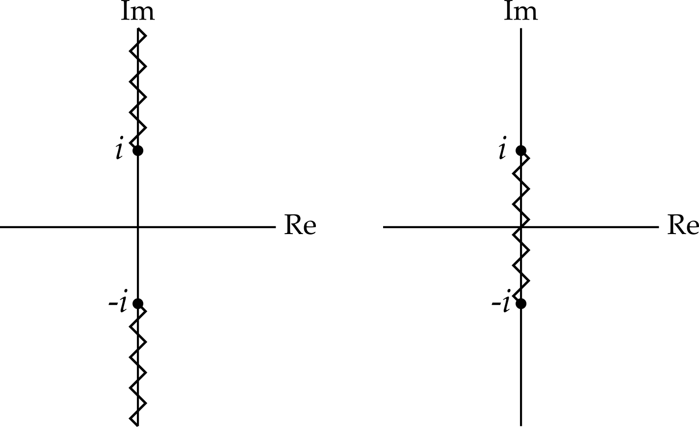
Exercise

Convince yourself that, in each case, the branch cuts ‘forbid’ those paths that encircle one, but not both of the branch points. (Note that both choices also forbid some paths that could have been accommodated with a different placement of branch cuts.)