7 The Cauchy formula and power series
7.1 Cauchy’s integral formula
Theorem 7.1 (Cauchy’s integral formula) If \(f(z)\) is holomorphic on and within a closed contour \(\gamma\) and \(z_0\) is a point within \(\gamma\), then \[ \boxed { \oint_\gamma \frac{f(z)}{z - z_0}\,dz = 2\pi if(z_0). } \]
Proof. Consider \(f(z)\) holomorphic on and within contour \(\gamma\).
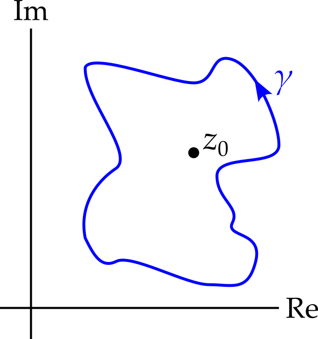
Note that the integrand, \(f(z) / (z - z_0)\), can only be holomorphic at \(z = z_0\) in the unlikely case that \(f(z_0) = 0\). So, we cannot use Cauchy’s theorem directly but we can deform the contour to a circle of radius \(\rho\) centred at \(z = z_0\), without the contour ever crossing \(z = z_0\). By doing so, we simplify the contour without changing the value of the integral.
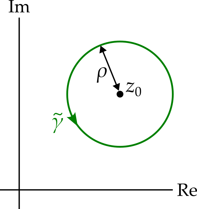
We can now evaluate the integral. For points on \(\widetilde{\gamma}\) we write \(z = z_0 + \rho e^{i\theta}\) and get \(dz = i\rho e^{i\theta}\), so \[ \begin{aligned} \oint_\gamma \frac{f(z)}{z - z_0}\,dz &= \oint_{\widetilde{\gamma}} \frac{f(z)}{z - z_0}\,dz\\ &= \int_0^{2\pi} \frac{f(z_0 + \rho e^{i\theta})}{\rho e^{i\theta}}.i\rho e^{i\theta}\,d\theta\\ &= i\int_0^{2\pi} f(z_0 + \rho e^{i\theta})\,d\theta \end{aligned} \tag{7.1}\] We now consider a shrinking radius, \(\rho \rightarrow 0\). We would like to say that, as \(\rho\) approaches zero, \(f(z_0 + \rho e^{i\theta}) \rightarrow f(z_0)\) (since \(f\) is continuous) and hence \[ \lim_{\rho \rightarrow 0}\left(i\int_0^{2\pi} f(z_0 + \rho e^{i\theta})\,d\theta\right) = i\int_0^{2\pi} f(z_0)\,d\theta = 2\pi if(z_0). \] Since the value of the integral does not change during this process, it must be the case that \[ \oint_\gamma \frac{f(z)}{z - z_0}\,dz = 2\pi if(z_0) \] as required.
In an exam, I wouldn’t expect any more detail than given above. However, you might have concerns about the step where we take the limit, so let’s prove this in a little more detail. This will also give us a chance to use some results and definitions seen earlier in the course.
Given that \(f(z_0)\) is constant, we have \[ 2\pi if(z_0) = i\int_0^{2\pi}f(z_0)\,d\theta \] Subtract this from our previous result, equation 7.1, and take the size of both sides: \[ \begin{aligned} \left|\int_{\widetilde{\gamma}} \frac{f(z)}{z - z_0}\,dz - 2\pi if(z_0)\right| &= \left|i\int_0^{2\pi} f(z_0 + \rho e^{i\theta})\,d\theta - i\int_0^{2\pi}f(z_0)\,d\theta\right|\\ &= \left|\int_0^{2\pi}\left(f(z_0 + \rho e^{i\theta}) - f(z_0)\right)d\theta\right| \end{aligned} \] Now since \(f\) is continuous at \(z = z_0\), given \(\epsilon > 0\) we can ensure that \(\left|f(z_0 + \rho e^{i\theta}) - f(z_0)\right| < \epsilon\) by choosing a small enough value for \(\rho\). Using our useful result, equation 6.1, from section 6.2.1, we now get \[ \begin{aligned} \left|\int_{\widetilde{\gamma}} \frac{f(z)}{z - z_0}\,dz - 2\pi if(z_0)\right| &= \left|\int_0^{2\pi}\left(f(z_0 + \rho e^{i\theta}) - f(z_0)\right)d\theta\right| \leq 2\pi\epsilon \end{aligned} \] Since we can choose \(\epsilon\) as small as we wish, this difference approaches zero as \(\rho \rightarrow 0\). Hence, \[ \lim_{\rho \rightarrow 0}\int_{\widetilde{\gamma}} \frac{f(z)}{z - z_0}\,dz = 2\pi if(z_0). \] Given that the value of the integral does not change, either in the initial deformation of the contour or in taking the limit, this means that \[ \int_\gamma \frac{f(z)}{z - z_0}\,dz = 2\pi if(z_0) \] as required.
What does Cauchy’s integral formula tell us? It can be viewed in two ways. Firstly, the formula is useful for quickly evaluating certain integrals on closed paths1.
1 This will be superceded later by the Residue Theorem, which will allow us to quickly evaluate a much wider range of integrals.
Calculate \[ \oint_\gamma \frac{e^z}{z - 2}\,dz \] over the two contours shown.
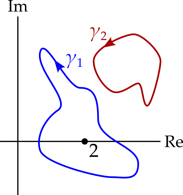
For contour \(\gamma_1\), we use the integral formula, setting \(f(z) = e^z\) and \(z_0 = 2\), giving us \[ \oint_{\gamma_1} \frac{e^z}{z - 2}\,dz = 2\pi if(z_0) = 2\pi ie^2. \] For contour \(\gamma_2\), we simply note that the integrand is holomorphic both on and inside the contour. Hence \[ \oint_{\gamma_2} \frac{e^z}{z - 2}\,dz = 0 \] by Cauchy’s theorem.
Secondly, we may view Cauchy’s integral formula in reverse, as a formula for the values of \(f\) inside the contour \(\gamma\), i.e. \[ f(z) = \frac{1}{2\pi i}\oint_\gamma \frac{f(w)}{w - z}\,dw. \tag{7.2}\] Surprisingly, this tells us that if the values of a holomorphic function \(f\) are known on a closed contour, then this automatically fixes the \(f\) at all interior points. There is no flexibility - any deviation from the formula, at any interior points will make the function non-holomorphic.
7.2 Cauchy’s integral formula for derivatives
Looking at equation 7.2, we see that the integral is with respect to \(w\), so provided the integrand is well-behaved2, we should be able to differentiate \(f(z)\) by differentiating ‘under the integral sign’. \[ \begin{aligned} f'(z) &= \frac{d}{dz}\left(\frac{1}{2\pi i}\oint_\gamma \frac{f(w)}{w - z}\,dw\right)\\ &= \frac{1}{2\pi i}\oint_\gamma f(w)\frac{d}{dz}\frac{1}{w - z}\,dw\\ &= \frac{1}{2\pi i}\oint_\gamma \frac{f(w)}{(w - z)^2}\,dw. \end{aligned} \] Repeating the process, we find that \[ \boxed { f^{(n)}(z) = \frac{n!}{2\pi i}\oint_\gamma \frac{f(w)}{(w - z)^{n + 1}}\,dw. } \] This is the generalised Cauchy integral formula.
2 I will not provide the details here. For more information, look up ‘Leibniz integral rule’ or ‘differentiation under the integral sign’. You may also come across ‘Feynman’s trick’ for using the rule as a method of evaluating integrals.
3 Compare this with the case for functions on the real numbers.
Notice that this implies that, if \(f\) is differentiable on and within the contour \(\gamma\), then this is sufficient to ensure the existence of derivatives of all orders3.
Calculate \[ \oint_\gamma \frac{e^z}{(z - 2)^3}\,dz \] over the two contours shown.
For contour \(\gamma_1\), we use the integral formula for \(f''(z)\), with \(f(z) = e^z\) and \(z_0 = 2\). Since \(f''(z) = e^z\), this gives us \[ e^2 = \frac{2}{2\pi i}\oint_{\gamma_1} \frac{e^w}{(w - 2)^3}\,dw \] and so \[ \oint_{\gamma_1}\frac{e^z}{(z - 2)^3}\,dz = \pi ie^2. \]
as in the previous example, the integrand is holomorphic on and inside the contour \(\gamma_2\), so by Cauchy’s theorem \[ \oint_{\gamma_2} \frac{e^z}{(z - 2)^3}\,dz = 0 \] by Cauchy’s theorem.
7.3 Taylor series
Consider the following two questions.
- If \(f : \mathbb{R}\rightarrow\mathbb{R}\) is well-behaved in an interval \(I = (a - R, a + R)\), can we always find a Taylor series that approaches \(f\) in all of the interval?
- If \(f : \mathbb{C}\rightarrow\mathbb{C}\) is well-behaved in a disk D = \(\{z : \left|z - a\right| < R\}\), can we always find a Taylor series that approaches \(f\) in all of the disk?
The answer to question 1 is, unfortunately, “no”. We have already considered the function \(f(x) = 1 / (1 + x^2)\) in an examples class. It is a very well behaved function over all of \(\mathbb{R}\), with continuous derivatives of any order, yet its Taylor series is \[ \frac{1}{1 + x^2} = 1 - x^2 + x^4 - x^6 + \ldots, \] which clearly diverges when \(\left|x\right| > 1\)
We will now demonstrate that the answer to question 2 is “yes”.
Fix \(z \in D\), choose \(r\) such that \(\left|z - a < r < R\right|\) and let \(\gamma\) be the circle of radius \(r\) about point \(a\).
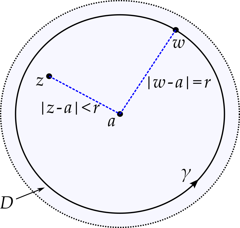
We now apply Cauchy’s integral formula to get \[ \begin{aligned} f(z) &= \frac{1}{2\pi i}\oint_\gamma \frac{f(w)}{w - z}\,dw\\ &= \frac{1}{2\pi i}\oint_\gamma \frac{f(w)}{(w - a) - (z - a)}\,dw\\ &= \frac{1}{2\pi i}\oint_\gamma \frac{f(w)}{w - a}.\frac{w - a}{(w - a) - (z - a)}\,dw\\ &= \frac{1}{2\pi i}\oint_\gamma \frac{f(w)}{w - a}.\frac{1}{\left(1 - (z - a)/(w - a)\right)}\,dw.\\ \end{aligned} \]
Noting4 that \(\left|(z - a)/(w - a)\right| < 1\), we recognize that the second factor in the integrand is the sum of a geometric series. \[ \frac{1}{\left(1 - (z - a)/(w - a)\right)} = \sum_{n = 0}^\infty \left(\frac{z - a}{w - a}\right)^n. \] So we have \[ f(z) = \frac{1}{2\pi i}\oint_\gamma \frac{f(w)}{w - a}\sum_{n = 0}^\infty \left(\frac{z - a}{w - a}\right)^n\, dw. \]
4 Here it is essential that both the region \(D\) and the contour \(\gamma\) are circular.
5 This may seem reasonable, but it is not obvious that we can safely do this. I omit the technical detail of this step here - it depends upon the fact the that series is uniformly convergent - a concept from real analysis.
Switching the order of the summation and the integration5, this becomes \[ f(z) = \sum_{n = 0}^\infty (z - a)^n\frac{1}{2\pi i}\oint_\gamma \frac{f(w)}{(w - a)^{n + 1}}\, dw. \] The integral does not depend on \(z\), so we can write this as \[ f(z) = \sum_{n = 0}^\infty p_n(z - a)^n \] where \[ p_n = \frac{1}{2\pi i}\oint_\gamma \frac{f(w)}{(w - a)^{n + 1}}\, dw. \] This certainly looks like a Taylor series expansion about \(z = a\). The only remaining difficulty is that the coefficients \(p_n\) should not depend on \(z\), yet the choice of contour \(\gamma\) does. However, we can use the generalised Cauchy integral formula to see that \[ p_n = \frac{f^{(n)}(a)}{n!} \] and we now have the more familiar form of the Taylor series, \[ f(z) = \sum_{n = 0}^\infty \frac{f^{(n)}(a)}{n!}(z - a)^n, \] with coefficients that do not depend on \(z\).
7.3.1 Radius of convergence
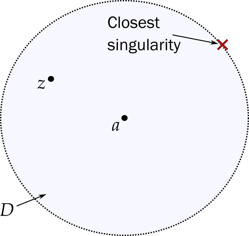
We have a Taylor series that works in region \(D\). Might the series work in a larger region?
We can expand the circular region \(D\), while maintaining its circular shape, and so long as no singularities are introduced6, the same argument can be repeated in the larger region. Hence the Taylor series works in a disk that extends to the closest singularity of \(f\).
6 I.e. as long as \(f\) remains holomorphic in \(D\).
Example 7.1 Expand \(f(z) = 1 / z^2\) in a Taylor series about the point \(z_0 = 1\) and find the radius of convergence.
We could find the Taylor series by other methods7, but here we calculate derivatives at \(z_0 = 1\).
7 Find the Taylor series of \(1/z\) about \(z_0 = 1\) by comparing with the geometric series, then differentiate.
| \(n\) | \(f^{(n)}(z)\) | \(f^{(n)}(1)\) | \(\frac{f^{(n)}(1)}{n!}\) |
|---|---|---|---|
| \(0\) | \(\frac{1}{z^2}\) | \(1\) | \(1\) |
| \(1\) | \(\frac{-2}{z^3}\) | \(-2\) | \(-2\) |
| \(2\) | \(\frac{6}{z^4}\) | \(6\) | \(3\) |
| \(3\) | \(\frac{-24}{z^5}\) | \(-24\) | \(-4\) |
| \(\vdots\) | \(\vdots\) | \(\vdots\) | \(\vdots\) |
| \(k\) | \(\frac{(-1)^k(k + 1)!}{z^{k + 2}}\) | \((-1)^k(k + 1)!\) | \((-1)^k(k + 1)\) |
The required Taylor series is therefore \[ \begin{aligned} f(z) = \frac{1}{z^2} &= \sum_{n = 0}^\infty (-1)^n(n + 1)(z - 1)^n\\ &= \sum_{n = 0}^\infty (n + 1)(1 - z)^n\\ &= 1 + 2(1 - z) + 3(1 - z)^2 + 4(1 - z)^3 + \ldots \end{aligned} \] Using the ratio test, we can show that the series converges provided \(\left|1 - z\right| < 1\). Notice that this is precisely the distance from \(z_0 = 1\) to the singularity at \(z = 0\).
Determine the radius of convergence of the Taylor series for \(f(z) = 1 / (1 + z^2)\) about the point \(z_0 = 0\).
You will have found the Taylor series for \(f(z)\) in the examples class, by comparison with the geometric series. However, to answer the question, we do not need to calculate the series. We need only determine the distance from \(z_0 = 0\) to the nearest singularity. Since \(f(z)\) has singularities at \(z = \pm i\), the radius of convergence equals one.
7.4 Laurent series
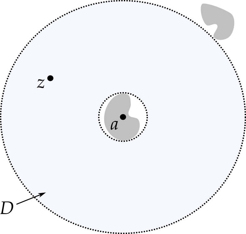
We have seen how a function has a Taylor series in a circular region, provided the function is holomorphic there. But what about if the function has some singularities in the region? Suppose a function is known to be holomorphic in an annulus (ring) as illustrated in figure 7.8.
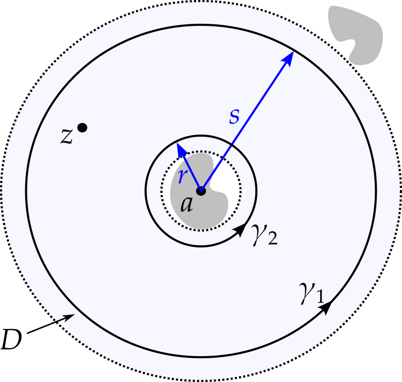
Theorem 7.2 (Laurent series) Suppose function \(f\) is holomorphic in the region \[ D = \{z \in \mathbb{C} : R < \left|z - a\right| < S\}. \] Then \[ f(z) = \sum_{n = -\infty}^\infty c_n(z - a)^n, \] where \[ c_n = \frac{1}{2\pi i}\int_\gamma \frac{f(w)}{(w - a)^{n + 1}}\,dw \] and \(\gamma\) is any path within the region \(D\) that circles \(a\) once, anticlockwise.
Proof. Consider a point \(z \in D\). We can choose \(r\) and \(s\) to satisfy \(R < r < \left|z - a\right| < s < S\), so that circles of radii \(r\) and \(s\) lie within \(D\) and \(z\) lies between the two circles.
Now create a contour by creating a ‘channel’ between the two circles as shown in figure 7.10.
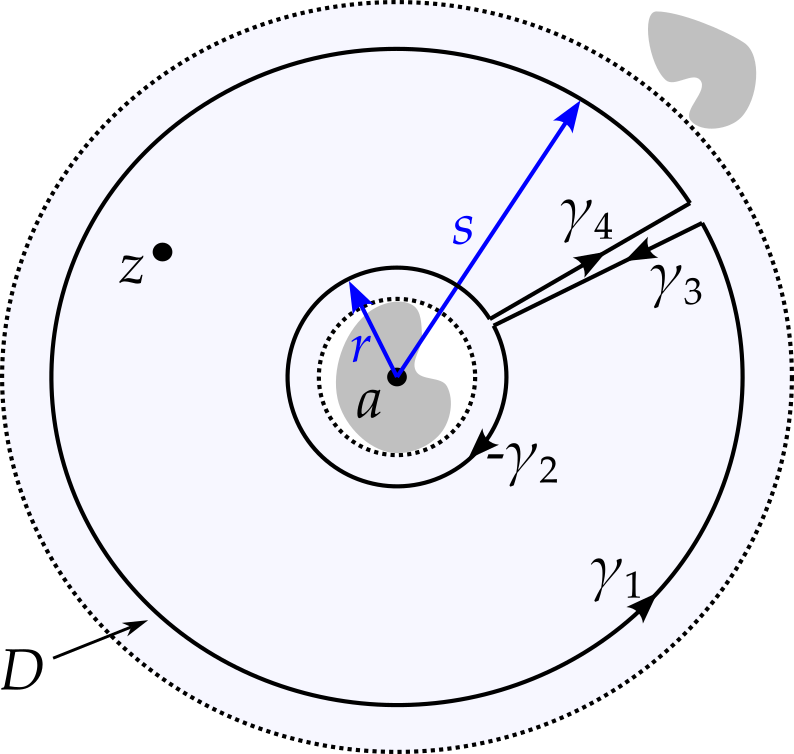
We can now use the Cauchy integral theorem to find \(f(z)\), since \(f\) is holomorphic on and within the contour. Hence \[ \begin{aligned} f(z) &= \frac{1}{2\pi i}\oint_{\gamma_1 + \gamma_3 - \gamma_2 + \gamma_4} \frac{f(w)}{w - z}\,dw\\ &= \frac{1}{2\pi i}\oint_{\gamma_1} \frac{f(w)}{w - z}\,dw - \frac{1}{2\pi i}\oint_{\gamma_2} \frac{f(w)}{w - z}\,dw\\ &\qquad\qquad + \frac{1}{2\pi i}\oint_{\gamma_3} \frac{f(w)}{w - z}\,dw + \frac{1}{2\pi i}\oint_{\gamma_4} \frac{f(w)}{w - z}\,dw. \end{aligned} \] Take the limit as the channel becomes narrower, so that \(\gamma_4\) becomes the same path as \(\gamma_3\), but in reverse. The integrals along these two segments cancel to leave \[ f(z) = f_1(z) + f_2(z) \] where \[ f_1(z) = \frac{1}{2\pi i}\oint_{\gamma_1} \frac{f(w)}{w - z}\,dw,\qquad f_2(z) = -\frac{1}{2\pi i}\oint_{\gamma_2} \frac{f(w)}{w - z}\,dw. \] For the first integral, we employ the same trick as we used for Taylor’s theorem. We note that \[ \frac{1}{w - z} = \frac{1}{(w - a) - (z - a)} = \frac{1}{w - a}.\frac{1}{1 - (z - a)/(w - a)} \] and note that, on \(\gamma_1\), \(\left|z - a\right| < \left|w - a\right|\), meaning that the second factor can be expanded as a geometric series. Hence \[ \frac{1}{w - z} = \frac{1}{w - a}\sum_{n = 0}^\infty\left(\frac{z - a}{w - a}\right)^n = \sum_{n = 0}^\infty\frac{(z - a)^n}{(w - a)^{n + 1}} \] and so \[ \begin{aligned} f_1(z) &= \frac{1}{2\pi i}\oint_{\gamma_1}f(w)\sum_{n = 0}^\infty\frac{(z - a)^n}{(w - a)^{n + 1}}\,dw\\ &= \sum_{n = 0}^\infty (z - a)^n \frac{1}{2\pi i}\oint_{\gamma_1}\frac{f(w)}{(w - a)^{n + 1}}\,dw \end{aligned} \tag{7.3}\] Notice that this is the usual Taylor series that converges for all \(z\) inside \(\gamma_1\).
For the second integral, we start by noting that \[ f_2(z) = -\frac{1}{2\pi i}\oint_{\gamma_2} \frac{f(w)}{w - z}\,dw = \frac{1}{2\pi i}\oint_{\gamma_2} \frac{f(w)}{z - w}\,dw. \] We now proceed in a similar manner to before, but with \(z\) and \(w\) switched. We see that \[ \frac{1}{z - w} = \frac{1}{(z - a) - (w - a)} = \frac{1}{z - a}.\frac{1}{1 - (w - a)/(z - a)} \] and note that on \(\gamma_2\), \(\left|w - a\right| < \left|z - a\right|\). We again recognise a geometric series and get \[ \frac{1}{z - w} = \frac{1}{z - a}\sum_{n = 0}^\infty \left(\frac{w - a}{z - a}\right)^n = \sum_{n = 0}^\infty \frac{(w - a)^n}{(z - a)^{n + 1}} \] Hence \[ \begin{aligned} f_2(z) &= \frac{1}{2\pi i}\oint_{\gamma_2}f(w)\sum_{n = 0}^\infty \frac{(w - a)^n}{(z - a)^{n + 1}}\,dw\\ &= \sum_{n = 0}^\infty (z - a)^{-n - 1}\frac{1}{2\pi i}\oint_{\gamma_2}\frac{f(w)}{(w - a)^{-n}}\,dw\\ &= \sum_{n = -\infty}^{-1}(z - a)^n\frac{1}{2\pi i}\oint_{\gamma_2}\frac{f(w)}{(w - a)^{n + 1}}\,dw \end{aligned} \tag{7.4}\] where we have relabelled the indices in the last step. We now note that the integrands in both equation 7.3 and 7.4 are holomorphic within the annulus. Hence the contours can be deformed into any contour, \(\gamma\), within the annulus that circles \(a\) once anticlockwise, without changing the result. We therefore get \[ f(z) = \sum_{n = -\infty}^{\infty}(z - a)^n\frac{1}{2\pi i}\oint_{\gamma} \frac{f(w)}{(w - a)^{n + 1}}. \] This can be written as \[ f(z) = \sum_{n = -\infty}^\infty c_n(z - a)^n, \] where \[ c_n = \frac{1}{2\pi i}\int_\gamma \frac{f(w)}{(w - a)^{n + 1}}\,dw. \]
7.4.1 Finding Laurent series
When finding Taylor series about \(z = a\), while it is sometimes more convenient to exploit our knowledge of geometric and other known series, we can always fall back on the method of calculating derivatives of \(f(z)\) at \(z = a\). For Laurent series, on the other hand, calculating \[ c_n = \frac{1}{2\pi i}\int_\gamma \frac{f(w)}{(w - a)^{n + 1}}\,dw \] might be challenging. It is therefore important to know and be able to manipulate known Taylor series when attempting to find the Laurent series for a function. The following examples will illustrate.
Example 7.2 Expand \(f(z) = 1 / (z - 1)^2\) about \(a = 1\).
Here \(f(z)\) has a singularity at \(z = 1\), so it will not be possible to find a Taylor series. We will need a Laurent series. However, a moments thought should reveal that this already is a Laurent series, with coefficients \(c_{-2} = 1\) and \(c_n = 0\) for \(n \neq -2\).
Example 7.3 Expand \(f(z) = e^z / z^2\) about \(a = 0\).
This function has a singularity at \(z = 0\), so we will need a Laurent series. Recall that \[ e^z = \sum_{n = 0}^\infty \frac{z^n}{n!} = 1 + z + \frac{z^2}{2} + \frac{z^3}{6} + \ldots \] Hence \[ \frac{e^z}{z^2} = \sum_{n = 0}^\infty \frac{z^{n - 2}}{n!} = z^{-2} + z^{-1} + \frac{1}{2} + \frac{z}{6} + \ldots \]
Example 7.4 Expand \(\displaystyle f(z) = \frac{1}{z(1 + z^2)}\) about \(a = 0\).
Here \(f(z)\) has singularities at \(z = 0\) and at \(z = \pm i\). There are therefore two regions to be considered: region \(A\) where \(0 < \left|z\right| < 1\) and region \(B\) where \(\left|z\right| > 1\)
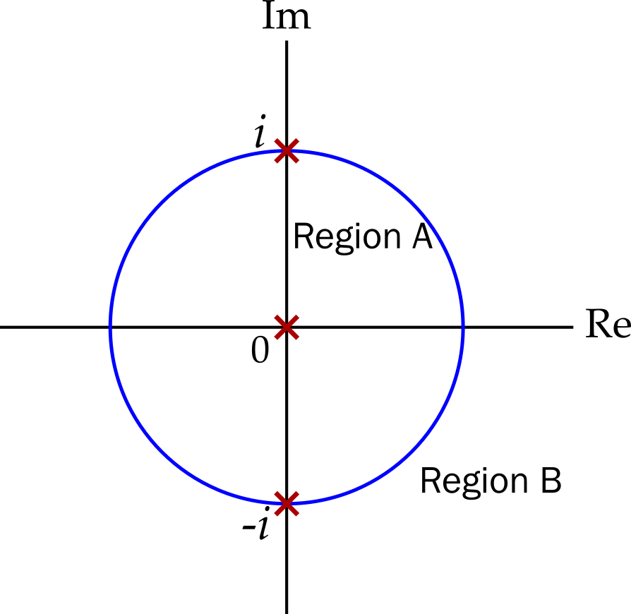
In region \(A\), we write \[ \begin{aligned} f(z) &= \frac{1}{z}.\frac{1}{1 + z^2}\\ &= \frac{1}{z}\sum_{n = 0}^\infty (-z^2)^n\\ &= \frac{1}{z}(1 - z^2 + z^4 - z^6 + \ldots)\\ &= \frac{1}{z} - z + z^3 - z^5 + \ldots \end{aligned} \] i.e. in region \(A\) \[ f(z) = \sum_{n = 0}^\infty(-1)^nz^{2n - 1}. \]
In region \(B\), the Taylor series for \(1 / (1 + z^2)\) no longer works. We need a series that will work when \(\left|z\right|\) is large and hence when \(1/\left|z\right|\) is small, i.e. a series in \(1/z\). So \[ \begin{aligned} f(z) &= \frac{1}{z}.\frac{1}{1 + z^2}\\ &= \frac{1}{z^3}.\frac{1}{1 + 1/z^2}\\ &= \frac{1}{z^3}\sum_{n = 0}^\infty \left(-\frac{1}{z^2}\right)^n\\ &= \frac{1}{z^3}\left(1 - \frac{1}{z^2} + \frac{1}{z^4} - \frac{1}{z^6} + \ldots\right)\\ &= \frac{1}{z^3} - \frac{1}{z^5} + \frac{1}{z^7} - \frac{1}{z^9} + \ldots \end{aligned} \]