Real versus complex differentiability

Different notions of differentiability

If you are used to equating ‘differentiable’ with ‘smoothly varying’, then the complex derivative might be a little unsettling. After all, \(f(z) = \left|z\right|^2 = z^*z\) is smoothly varying, as is \(g(z) = \operatorname{Re}z\), but neither of these functions is (complex) differentiable. It may be helpful to know that there are two notions of differentiability. Real differentiability captures the notion of ‘smoothly varying’, while complex differentiability is more restrictive, but turns out to be more useful.

In this appendix, we will explore what it means for a complex function to be ‘real’ differentiable and look at the difference between the two notions of differentiability. In doing so, we will treat complex number as numbers, as 2d vectors and as \(2\times2\) matrices.

Real differentiability

What makes \(\mathbb{C}\) different from the 2-dimensional space \(\mathbb{R}^2\)? Just one thing - the rule for multiplying complex numbers. Let’s forget this rule for a while and treat complex numbers \(z\) and \(f(z)\) as the vectors

\[ \mathbf{x} = \begin{pmatrix} x\\ y \end{pmatrix} \quad \text{and} \quad \mathbf{f}(\mathbf{x}) = \begin{pmatrix} u(x, y)\\ v(x, y) \end{pmatrix}. \] What does it mean for \(\mathbf{f}\) to be differentiable¹ at \(\mathbf{x}\)?

¹ You have seen various different derivatives of vector functions, e.g. partial derivatives, the gradient, the divergence, etc., but you may be less familiar with the derivative. This is sometimes called the total derivative.

It will be useful for us to look at a slightly more general case, where \(\mathbf{x}\) is a \(m\)-dimensional vector and \(\mathbf{f}\) is a function from \(\mathbb{R}^m\) to \(\mathbb{R}^n\).

Definition 1 We would like to find something - let’s call it \(\frac{d\mathbf{f}}{d\mathbf{x}}\) - that satisfies² \[ \delta\mathbf{f} \simeq \frac{d\mathbf{f}}{d\mathbf{x}}\delta\mathbf{x} \tag{1}\] for any small change, \(\delta\mathbf{x}\), to the input, \(\mathbf{x}\), where \(\delta\mathbf{f}\) is the resulting change in the output of the function \(\mathbf{f}\). If we can find such an object then we call it the derivative of \(\mathbf{f}\) at \(\mathbf{x}\) and say that \(\mathbf{f}\) is differentiable at \(\mathbf{x}\). We will also write the derivative of \(\mathbf{f}\) at \(\mathbf{x}\) as \(\mathbf{f}'(\mathbf{x})\).³

² What do we mean by \(\simeq\) here? Well, we want the error in this equation to approach zero faster than \(\delta\mathbf{x}\) as \(\delta\mathbf{x} \rightarrow 0\).

³ Other notations include \(d\mathbf{f}_{\mathbf{x}}\), \(D\mathbf{f}_{\mathbf{x}}\) and \(D\mathbf{f}(\mathbf{x})\). I have chosen the notations most similar to those we use for the complex derivative.

What could \(\frac{d\mathbf{f}}{d\mathbf{x}}\) be? It must be something that, when applied to the \(m\)-dimensional vector \(\mathbf{x}\), produces an \(n\)-dimensional vector \(\mathbf{f}(\mathbf{x})\). It must be an \(n\times m\) matrix.

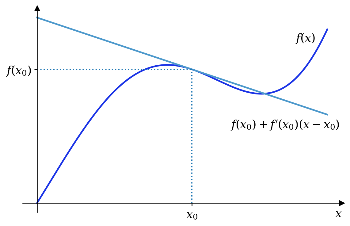
Example 1 If \(m = n = 1\), then the derivative at, for example, \(x = x_0\), is a \(1\times1\) matrix, i.e. just the number \(f'(x_0)\). Equation 1 then states that near \(x = x_0\) the function is approximated by the tangent at that point.

Figure 1: The derivative illustrated for \(f: \mathbb{R} \rightarrow \mathbb{R}\). The function \(f(x)\) is illustrated by the dark blue line while the straight line shows the linear approximation \(f(x_0) + f'(x_0)(x - x_0)\), equivalent to equation 1.

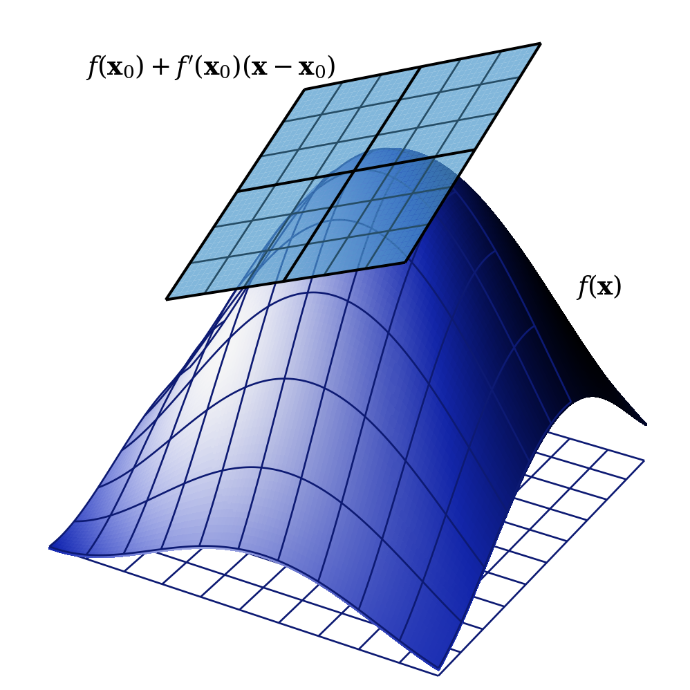
Example 2 For \(m = 2\) and \(n = 1\), the derivative is a two-element row vector — the gradient, \(\nabla f\), of \(f\) — and equation 1 indicates that, near to \(\mathbf{x}_0\), \(f(\mathbf{x})\) is approximated by a plane.

Figure 2: The derivative illustrated for \(f: \mathbb{R}^2 \rightarrow \mathbb{R}\). The function \(f(x)\) is illustrated by the dark blue surface while the plane shows the linear approximation \(f(\mathbf{x}_0) + f'(\mathbf{x}_0)(\mathbf{x} - \mathbf{x}_0)\), equivalent to equation 1.

Unfortunately, creating a similar diagram for the case we are most interested in, i.e. when \(m = n = 2\), is challenging, since it would require 4-dimensions. In this case the derivative is a \(2\times2\) matrix and we can find the components of the matrix by considering \(\delta\mathbf{x}\) in directions parallel to the axes. For example, suppose that \[ \delta\mathbf{x} = \begin{pmatrix} \delta x\\ 0 \end{pmatrix}. \] Writing \[ \frac{d\mathbf{f}}{d\mathbf{x}} = \begin{pmatrix} D_{11} & D_{12}\\ D_{21} & D_{22} \end{pmatrix} \] we find that equation 1 becomes \[ \begin{pmatrix} \delta u\\ \delta v \end{pmatrix} \simeq \begin{pmatrix} D_{11} & D_{12}\\ D_{21} & D_{22} \end{pmatrix} \begin{pmatrix} \delta x\\ 0 \end{pmatrix} = \begin{pmatrix} D_{11}\delta x\\ D_{21}\delta x \end{pmatrix} \] Noting that \(y\) is held constant here, the first row gives us \(D_{11} = \frac{\partial u}{\partial x}\) and the second gives us \(D_{21} = \frac{\partial v}{\partial x}\). If we hold \(x\) constant instead, we find the second column of the matrix and obtain \[ \frac{d\mathbf{f}}{d\mathbf{x}} = \begin{pmatrix} \frac{\partial u}{\partial x} & \frac{\partial u}{\partial y}\\ \frac{\partial v}{\partial x} & \frac{\partial v}{\partial y} \end{pmatrix}. \tag{2}\] If we now expand equation 1, we get the comforting \[ \delta u = \frac{\partial u}{\partial x}\delta x + \frac{\partial u}{\partial y}\delta y \] and \[ \delta v = \frac{\partial v}{\partial x}\delta x + \frac{\partial v}{\partial y}\delta y, \] i.e. the chain rule.

Now, the existence of partial derivatives ensures that we can create the matrix in equation 2, but is this enough to ensure that it is the derivative, i.e. that equation 1 holds? Not quite. Consider the function \(f : \mathbb{R}^2 \rightarrow \mathbb{R}\) defined by \[ f(\mathbf{x}) = f\begin{pmatrix}x\\y\end{pmatrix} = \begin{cases} 1 & \text{if } x = 0,\\ 1 & \text{if } y = 0,\\ 0 & \text{otherwise.} \end{cases} \] This has partial derivatives at the origin, where \(\frac{\partial f}{\partial x} = \frac{\partial f}{\partial y} = 0.\) However, it is not true that \[ \delta f \simeq \begin{pmatrix} \frac{\partial f}{\partial x} & \frac{\partial f}{\partial y} \end{pmatrix} \begin{pmatrix} \delta x\\ \delta y \end{pmatrix} = \frac{\partial f}{\partial x}\delta x + \frac{\partial f}{\partial y}\delta y \] for any small \(\delta \mathbf{x}\). Here the right hand side is zero, whereas if \(\delta\mathbf{x}\) is not parallel to one of the axes we find that \(\delta f = -1\). It is for this reason that the partial derivatives must not only exist, but must also be continuous in a neighbourhood of \(\mathbf{x}\). (I will not prove that this is sufficient for differentiability here.)

Example 3 Consider finding the real derivative of complex function \(f(z) = z^*z\). In terms of vectors, this becomes \[ \mathbf{f}(\mathbf{x}) = \begin{pmatrix} x^2 + y^2\\ 0 \end{pmatrix}. \] If we refer to the two components of \(\mathbf{f}\) as \(u\) and \(v\), then partial derivatives certainly exist: \[ \frac{\partial u}{\partial x} = 2x, \qquad \frac{\partial u}{\partial y} = 2y, \] \[ \frac{\partial v}{\partial x} = 0, \qquad \frac{\partial v}{\partial y} = 0. \] Moreover, these partial derivatives are continuous and hence \(\mathbf{f}\) is real differentiable at \(\mathbf{x}\) with derivative \[ \frac{d\mathbf{f}}{d\mathbf{z}} = \begin{pmatrix} 2x & 2y\\ 0 & 0 \end{pmatrix} \] This corresponds with the notion that \(\mathbf{f}\) varies smoothly with \(\mathbf{x}\).

Detour: Complex numbers as matrices

We have seen that complex numbers can be thought of as 2-dimension vectors, if we forget about multiplication. Unfortunately, complex multiplication does not correspond with any of our notions of vector multiplication. We will now see that complex numbers may also be represented as \(2\times2\) matrices. Moreover, when represented in this way, matrix multiplication will correspond with complex multiplication.

Let’s look again at how complex multiplication works. If we think of complex numbers as 2d vectors, then multiplication by a fixed complex number \(w\) will map 2d vectors on to 2d vectors. Does this remind you of anything?

Let’s write \(wz\) in Cartesian form. \[ \begin{aligned} wz &= (\operatorname{Re}w + i\operatorname{Im}w)(\operatorname{Re}z + i\operatorname{Im}z)\\ &= \operatorname{Re}w \operatorname{Re}z - \operatorname{Im}w \operatorname{Im}z + i(\operatorname{Re}w \operatorname{Im}z + \operatorname{Im}w \operatorname{Re}z). \end{aligned} \] We can write this in matrix form, \[ \begin{pmatrix} \operatorname{Re}wz\\ \operatorname{Im}wz \end{pmatrix} = \begin{pmatrix} \operatorname{Re}w & -\operatorname{Im}w\\ \operatorname{Im}w & \operatorname{Re}w \end{pmatrix} \begin{pmatrix} \operatorname{Re}z\\ \operatorname{Im}z \end{pmatrix}. \tag{3}\] Here, complex multiplication is performed by writing \(wz\) and \(z\) as 2d vectors, but writing \(w\) as a \(2\times2\) real matrix, \[ w \leftrightarrow \begin{pmatrix} \operatorname{Re}w & -\operatorname{Im}w\\ \operatorname{Im}w & \operatorname{Re}w \end{pmatrix}. \] We will use this when we look again at complex differentiation.

There is, however, something a little unsatisfactory with equation 3: some complex numbers are represented by vectors, while others are represented by matrices. What happens if we rewrite equation 3 writing all the complex numbers as matrices? We get \[ \begin{pmatrix} \operatorname{Re}wz & -\operatorname{Im}wz\\ \operatorname{Im}wz & \operatorname{Re}wz \end{pmatrix} = \begin{pmatrix} \operatorname{Re}w & -\operatorname{Im}w\\ \operatorname{Im}w & \operatorname{Re}w \end{pmatrix} \begin{pmatrix} \operatorname{Re}z & -\operatorname{Im}z\\ \operatorname{Im}z & \operatorname{Re}z \end{pmatrix}, \] and look - the matrix multiplication still works correctly! Indeed, if we consider the set of matrices of the form \[ Z = \begin{pmatrix} x & -y\\ y & x \end{pmatrix} \] then we find that both matrix addition and matrix multiplication correspond with complex addition and multiplication.

Exercise

If we represent \(x + iy\) as the matrix \[ \begin{pmatrix} x & -y\\ y & x \end{pmatrix}, \] what does complex conjugation correspond with? Write \(e^{i\theta}\) in matrix form - do you recognise this matrix?

Solution

Complex conjugation of the complex number corresponds with taking the transpose of the matrix. Meanwhile, the complex number \(e^{i\theta}\) corresponds with \[ \begin{pmatrix} \cos\theta & -\sin\theta\\ \sin\theta & \cos\theta \end{pmatrix}, \] which you should recognise as a rotation by an angle of \(\theta\). This is, of course, what happens to a number in the complex plane when multiplied by \(e^{i\theta}\).

Complex differentiability

Let’s return to differentiability. We have shown that when complex numbers are treated as vectors, then the real derivative is a \(2\times2\) matrix. However, we want to be able to think of \(\mathbb{C}\) as a system of numbers, in which case derivatives that are \(2\times2\) real matrices are deeply unsatisfying. We want, for example, the derivative of complex function \(f(z) = e^z\) at \(z = z_0\) to be the complex number \(e^{z_0}\), not \[ \begin{pmatrix} e^{x_0}\cos y_0 & -e^{x_0}\sin y_0\\ e^{x_0}\sin y_0 & e^{x_0}\cos y_0 \end{pmatrix}. \] So we create a new notion - the complex derivative.

Definition 2 We wish to find a complex number, \(\frac{df}{dx}\), that satisfies \[ \delta f \simeq \frac{df}{dz}\delta z \tag{4}\] for any small change, \(\delta z\), to the input \(z\), where \(\delta f\) is the resulting change in the output of the function f. If we can find such a number then we call it the complex derivative of f at z.

The key difference here is that \(\frac{df}{dz}\) must be a complex number, not a matrix, and that the multiplication in equation 4 is complex multiplication, not matrix multiplication.

It should be clear that the notion of complex differentiability must be more restrictive than that of real differentiability. Why? Well, if \(\frac{df}{dz}\) must be a complex number, then we have only two real numbers - the real and imaginary parts - to play with, while \(\frac{d\mathbf{f}}{d\mathbf{x}}\) had four. Hence there will be functions that are differentiable in the real sense that are not complex differentiable.

We can see this more clearly if we write the complex multiplication of equation 4 in the form of equation 3. Writing \(\delta f = \delta u + i\delta v\) and \(\delta z = \delta x + i\delta y\), we get \[ \begin{pmatrix} \delta u\\ \delta v \end{pmatrix} = \begin{pmatrix} \operatorname{Re}\frac{df}{dz} & -\operatorname{Im}\frac{df}{dz}\\ \operatorname{Im}\frac{df}{dz} & \operatorname{Re}\frac{df}{dz} \end{pmatrix} \begin{pmatrix} \delta x\\ \delta y \end{pmatrix} \] This is in exactly the same form as equation 1, except that the matrix must correspond with a complex number. If the real derivative is of the form \[ Z = \begin{pmatrix} x & -y\\ y & x \end{pmatrix} \] then the complex derivative is \(x + iy\). If not, then the complex derivative does not exist.

Finally, let’s compare the matrix we have here with equation 2 for the real derivative. We get \[ \operatorname{Re}\frac{df}{dz} = \frac{\partial u}{\partial x} = \frac{\partial v}{\partial y} \] and \[ \operatorname{Im}\frac{df}{dz} = \frac{\partial v}{\partial x} = -\frac{\partial u}{\partial y} \] and lo and behold, we have the Cauchy-Riemann equations.