2  Complex functions

In this course we focus on the properties of complex-valued functions of a (single) complex variable, \(f : \mathbb{C} \rightarrow \mathbb{C}\). We know a wide range of real-valued functions of a real variable, \(f : \mathbb{R} \rightarrow \mathbb{R}\), e.g. \(f(x) = 1 + x^2\), \(f(x) = \sin x\), \(f(x) = 1 / (1 + e^x)\), \(f(x) = \cos(\log x)\), etc. How many of these can be converted to take complex arguments and return complex results? If we can convert functions such as \(f(x) = \sin x\) and \(f(x) = \cos x\) to take complex arguments, do they still follow the rules that we have become accustomed to?

In previous courses, we have successfully extended basic arithmetic operations to \(\mathbb{C}\) and we can confidently¹ add, subtract, multiply and divide complex numbers. We can therefore handle a range of complex functions such as polynomials, e.g. \(f(z) = z^4 - 2z^3 + z + 1\), and rational functions, e.g. \(f(z) = (z + 1) / (z^3 - z + 1)\), that are built up from simple arithmetic operations. Here we will look at the more complicated functions: powers and roots, exponentials, trigonometric functions and logarithms.

¹ Not so confident? I have provided a ‘chapter zero’ if you need to revise the basics of complex numbers.

2.1 Exponentials and trigonometric functions

2.1.1 The exponential function

We are hopefully all familiar with the polar representation of a complex number \[z = re^{i\theta} = r\cos\theta + ir\sin\theta.\] It is worth reminding ourselves of how we justified this, since here we have the exponential of an imaginary number. What does this mean? With \(e^{i\theta}\) previously undefined, we decided to interpret it as the result obtained by substituting \(i\theta\) into the Taylor expansion for \(e^x\), i.e. \[ \begin{split} e^{i\theta} &= 1 + i\theta + \frac{(i\theta)^2}{2!} + \frac{(i\theta)^3}{3!} + \frac{(i\theta)^4}{4!} + \frac{(i\theta)^5}{5!} + \ldots\\ &= 1 + i\theta - \frac{\theta^2}{2!} - i\frac{\theta^3}{3!} + \frac{\theta^4}{4!} + i\frac{\theta^5}{5!} - \ldots\\ &= 1 - \frac{\theta^2}{2!} + \frac{\theta^4}{4!} - \ldots + i\left(\theta - \frac{\theta^3}{3!} + \frac{\theta^5}{5!} - \ldots\right)\\ &= \cos\theta + i\sin\theta, \end{split} \] where in the last step, we recognised the Taylor expansions for \(\cos\theta\) and \(\sin\theta\).

This extends the definition of the exponential function to imaginary numbers, but there is no reason why we cannot use the power series to define the exponential function for all complex numbers². Hence we define \[e^z = \sum_{n = 0}^\infty \frac{z^n}{n!}\] for all complex \(z\).

² Or even other mathematical objects like matrices.

What properties does the exponential function have when we extend its domain of definition in this way? Well, it keeps almost all the properties that you are familiar with. We still have \[ \begin{aligned} e^we^z &= e^{w + z},\\ e^w / e^z &= e^{w - z},\\ e^{-z} &= 1 / e^z,\\ (e^w)^z &= e^{wz} \end{aligned} \] for \(w, z \in \mathbb{C}\) and since the values on the real axis are unchanged, we still have \(e^0 = 1\). We will later see that \(e^z\) is still continuous and that its derivative is still \(e^z\). The most notable difference is that \(e^z\) is no longer constrained to take only positive values. Indeed, \(e^z\) can take any complex value, with the exception of zero.

Exercise

Prove that \(e^we^z = e^{w + z}\) for any \(w, z \in \mathbb{C}\).

Solution

Start with \[e^we^z = \left(\sum_{l = 0}^\infty \frac{w^l}{l!}\right)\left(\sum_{m = 0}^\infty \frac{z^m}{m!}\right) = \sum_{l = 0}^\infty\sum_{m = 0}^\infty \frac{w^lz^m}{l!m!}.\] Now just consider those terms where \(l + m = n\), i.e. \[ \frac{w^n}{n!} + \frac{w^{n - 1}z}{(n - 1)!1!} + \frac{w^{n - 2}z^2}{(n - 2)!2!} + \ldots + \frac{z^n}{n!} = \sum_{m = 0}^n \frac{w^{n - m}z^m}{(n - m)!m!}. \] Multiply top and bottom by \(n!\) and we get \[ \frac{1}{n!}\sum_{m = 0}^n \frac{n!}{(n - m)!m!}w^{n - m}z^m = \frac{1}{n!}\sum_{m = 0}^n \binom{n}{m}w^{n - m}z^m. \] This should look familiar — recall the binomial theorem: \[ \left(w + z\right)^n = \sum_{m = 0}^n \binom{n}{m}w^{n - m}z^m. \] So adding all the terms where \(l + m = n\) gives us \((w + z)^n / n!\). Adding up all the terms must therefore give us \[ %e^we^z = \sum_{n = 0}^\infty \frac{(w + z)^n}{n!} \] which we recognise to be the Taylor expansion of \(e^{w + z}\). Hence \(e^we^z = e^{w + z}\).

2.1.2 Trigonometric functions

Much as for the exponential function, we could extend cosine and sine to complex numbers via their Taylor expansions. A simpler approach is to define them in terms of the exponential function. Start by assuming that Euler’s formula \[e^{i\theta} = \cos\theta + i\sin\theta\] works for complex values of \(\theta\). Hence, for complex number \(z\), we have \[ \begin{aligned} e^{iz} &= \cos z + i\sin z\\ e^{-iz} &= \cos z - i\sin z. \end{aligned} \] We can then solve these equations for \(\cos z\) and \(\sin z\), obtaining \[ \begin{aligned} \cos z &= \frac{e^{iz} + e^{-iz}}{2}\\ \sin z &= \frac{e^{iz} - e^{-iz}}{2i}. \end{aligned} \] These can then be our definitions of sine and cosine, from which we can obtain all the other trigonometric functions. Notice the similarity with the hyperbolic functions \[ \begin{aligned} \cosh z &= \frac{e^{z} + e^{-z}}{2}\\ \sinh z &= \frac{e^{z} - e^{-z}}{2}. \end{aligned} \]

As with the exponential function, trigonometric functions extended to the complex plane satisfy the usual equations, e.g. \(\sin^2z + \cos^2z = 1\), \(\cos2\theta = \cos^2\theta - \sin^2\theta\), etc. However, while the sine and cosine of real numbers can only take values between -1 and +1, when extended to the complex plane they can take any complex value. So, just as we can find a complex \(z\) that satisfies \(e^z = i\), we can also find \(z\) satisfying \(\cos z = 2\), provided we allow complex \(z\)

Exercise

Prove that \(\cos^2z + \sin^2z = 1\) for any \(z \in \mathbb{C}\).

Solution

First calculate \(\cos^2z\) and \(\sin^2z\): \[ \begin{aligned} \cos^2z &= \left(\frac{e^{iz} + e^{-iz}}{2}\right)^2 = \frac{1}{4}\left(e^{2iz} + 2 + e^{-2iz}\right)\\ \sin^2z &= \left(\frac{e^{iz} - e^{-iz}}{2i}\right)^2 = -\frac{1}{4}\left(e^{2iz} - 2 + e^{-2iz}\right) \end{aligned} \] Adding these together, all the \(e^{2iz}\) and \(e^{-2iz}\) terms cancel to leave \[ \cos^2z + \sin^2z = 1 \] as required.

2.2 Logarithms

Now that the exponential function can return any value except zero, we can take logarithms of any number except zero, even negative and complex numbers. Writing our complex number as \(z = re^{i\theta}\), and assuming that the logarithm³ follows the usual rules, we define \(\log z\) as follows. \[ \log z = \log\left(re^{i\theta}\right) = \log r + \log e^{i\theta} = \log r + i\theta. \] We will illustrate this with an example.

³ We use \(\log\) to mean the natural logarithm throughout these notes, i.e. the logarithm to base \(e\). In your physics education you will seldom need logarithms to base 10.

Example 2.1 Find the natural logarithm of \(z = 1 - i\).

To start, we need to write \(z\) in the form \(re^{i\theta}\), i.e. we need to find the modulus \(\left|z\right|\) and the argument \(\arg z\). The modulus is \(\left|z\right| = \sqrt{1^2 + (-1)^2} = \sqrt{2}.\)

The argument is a little trickier. We start by finding \(\arctan(-1 / 1)\). While we ought to know what angle has a tangent of -1, we find a calculator and get -0.7854 which is \(-\pi / 4\) radians. Before we assume that this is the argument⁴, we check that this value makes sense — looking at figure 2.1 we see that it does.

⁴ Recall that \(\tan\theta = \tan(\theta + \pi)\), so we need to check whether the value the calculator gives is the correct argument or whether we need to add or subtract \(\pi\).

Figure 2.1: Finding the argument of \(z = 1 - i\).

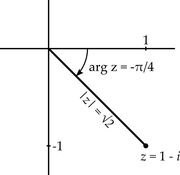
So \(z = \sqrt{2}e^{-\pi i/4}\). Taking the logarithm gives us \[\log(1 - i) = \log\left(\sqrt{2}e^{-\pi i/4}\right) = \log\sqrt{2} - \pi i/4.\]

2.2.1 The rise of multivaluedness

Hopefully the example above has helped you to understand how to take the logarithm of a complex number. However, you might have preferred to avoid negative angles and instead chosen the argument to be \(7\pi/4\) as shown in figure 2.2.

Figure 2.2: An alternative value for the argument of \(z = 1 - i\).

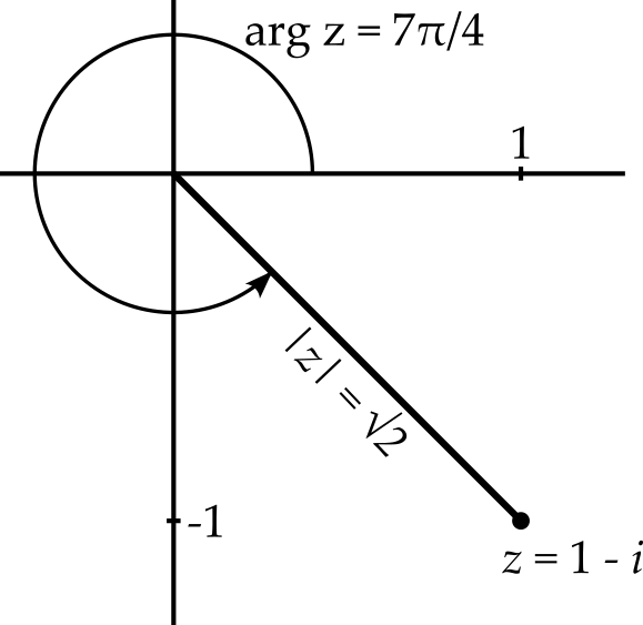
Let us run through the calculation again. We have \(z = \sqrt{2}e^{7\pi i/4}\). Taking the logarithm now gives us \[\log(1 - i) = \log\left(\sqrt{2}e^{7\pi i/4}\right) = \log\sqrt{2} + 7\pi i/4\] which differs from our previous result by \(2\pi i\). Which is correct?

Well, they both are! The logarithm is a multivalued function or multifunction. Indeed, we could add a further \(2\pi\) to \(7\pi/4\) to produce yet another possibility for the argument of \(1 - i\) and hence yet another possibility for the logarithm. Continuing this process reveals infinitely many possible values for the logarithm \[\log(1 - i) = \log\left(\sqrt{2}e^{7\pi i/4}\right) = \log\sqrt{2} + 2n\pi i - \pi i/4\] where \(n\) can be any integer.

Figure 2.3: Increasing the imaginary part of \(w = \log z\) results in an increase in the argument of \(z = e^w\). Eventually, the argument is increased by \(2\pi\), \(z\) returns to its original value and \(w\) is now at a new value for \(\log z\).

2.2.2 Principal value

While this holistic approach of treating the logarithm as a multifunction has some conceptual advantages, it can be useful to assign a single value⁵ to the complex logarithm, in much the same way as your calculator will always produce the positive square root, or always produce a value between \(-\pi/2\) and \(\pi/2\) when asked for the arctangent. We will see later that it may be advantageous to choose different assignments in different circumstances. However, the principal value for the argument and the logarithm is that value that satisfies the following constraints⁶: \[ -\pi < \operatorname{Arg}z \leq \pi, \] \[ -\pi < \operatorname{Im}(\operatorname{Log}z) \leq \pi. \]

⁵ The mathematical definition of a function requires that it be single valued, so the phrase ‘multivalued function’ is, in a sense, a contradiction.

⁶ Alas, there is not universal agreement, e.g. some sources define the principal value for the argument to be in \([0, 2\pi)\).

⁷ For those eagle-eyed readers who have spotted the possible ambiguity here, \(\log\sqrt{2}\) here refers to the normal, real-valued logarithm of \(\sqrt{2}\).

Different notational conventions are used to distinguish between a multivalued function and the principal value version. A common approach, used above, is to capitalise the principal valued function, so that \(\operatorname{Log}\) indicates the principal value of the logarithm \(\log\). Hence⁷ \[ \operatorname{Log}(1 - i) = \log\sqrt{2} - \pi i/4. \]

2.3 Powers and roots

If \(n\) is a positive integer then function \(f(z) = z^n\) can be defined simply via repeated multiplication, while we can also define \(z^{-n} = 1 / z^n\). Roots, i.e. \(z^{1/n}\) where \(n \in \mathbb{Z}\), can also be defined to be the number(s) that, when raised to the power of \(n\), return the value \(z\). But what about if \(n\) is an irrational number? What if \(n\) is complex?

The method that works for any value of \(n\) is simply to write \(z\) in polar form, i.e. \(z = re^{i\theta}\). Using the standard rules for exponentials, we then get \[ z^n = r^ne^{in\theta}. \] This formula is fine for any real \(n\), but if \(n\) is complex, what is \(r^n\)? Well, \(r^n = \left(e^{\log r}\right)^n = e^{n\log r}\) and we get \[ z^n = e^{n\log r}e^{in\theta} = e^{n(\log r + i\theta)} \] — a formula for calculating any power of \(z\).

Example 2.2 Calculate \((1 + i)^5\).

We could calculate this by repeated multiplication, but instead we will start by writing \(1 + i\) in polar form: \[1 + i = \sqrt{2}e^{\pi i / 4}.\] Raising this to the power of five is now straightforward \[(1 + i)^5 = \sqrt{2}^5e^{5\pi i/4} = 4\sqrt{2}e^{5\pi i/4} = 4(-1 - i).\]

Example 2.3 Calculate \((-i)^{1/2}\).

Writing \(-i = e^{-\pi i/2}\), we find that \[(-i)^{1/2} = e^{-\pi i/4} = \frac{1}{\sqrt{2}}(1 - i).\] But wait! We may also write \(-i = e^{3\pi i/2}\) and then we get \[(-i)^{1/2} = e^{3\pi i/4} = \frac{1}{\sqrt{2}}(-1 + i)\] — a different answer. This is the second square root of \(-i\). Can we find any more?

Suppose we add a further \(2\pi\) to the argument of \(-i\) to get \(-i = e^{7\pi i/2}\). Then we get \[(-i)^{1/2} = e^{7\pi i/4} = e^{-\pi i/4} = \frac{1}{\sqrt{2}}(1 - i)\] and we get our first result again. Therefore are there two square roots of \(-i\), \((1 - i) / \sqrt{2}\) and \((-1 + i) / \sqrt{2}\).

Which of these is the principal value? To obtain the principal value of \(z^n\), use the principal value for the argument of \(z\) when performing your calculation. In this case, we use \(\operatorname{Arg}(-i) = -\pi/2\), as we did in the first calculation and so the principal value of \((-i)^{1/2}\) is \((1 - i) / \sqrt{2}\).

Generally, when finding the \(n\)th roots, \(z^{1/n}\) of a complex number \(z\), we find that there are \(n\) such roots (unless \(z = 0\)). In other words, these are further examples of multivalued functions.

Example 2.4 Calculate \(i^i\).

Again, we express \(i\) in polar form, but suspecting that we might get multiple possible answers, we write \(i = e^{\pi i/2 + 2n\pi i}\), where \(n \in \mathbb{Z}\), i.e. we consider all possible values for the argument of \(i\) simultaneously. We get \[i^i = \left(e^{\pi i/2 + 2n\pi i}\right)^i = e^{-\pi/2 - 2n\pi}.\] Surprisingly, we find that the values of \(i^i\) are real!

What is the principal value? In the calculation use the principal value for the argument of \(i\), that is \(\operatorname{Arg}(i) = \pi i/2\) and obtain \[i^i = \left(e^{\pi i/2}\right)^i = e^{-\pi/2} \simeq 0.208.\]

2.4 Visualising complex functions

You will have learnt to plot and sketch graphs of real valued functions \(f: \mathbb{R} \rightarrow \mathbb{R}\) some years ago and have likely done this many times. Each real valued input \(x\) to function \(f\) produces a single output \(y = f(x)\). These combine to give the coordinates of a point in two dimensions. Joining these points appropriately produces your graph.

Now that we are considering complex valued functions of a complex variable, each input to the function is described by two real numbers, while two real numbers are also required to describe the functions output. Hence we need a 4-dimensional plot, which is a little more challenging. However, there are various methods that may be used.

• Domain colouring: Using the two dimensions of the plot for the input value, different colours can be used to represent different output values. Colours can be thought of as a three dimensional space⁸ — two of these dimensions can be used to illustrate the value. A common approach is to use the hue to represent the argument of the output and the lightness of the colour to represent the magnitude.

• Vector fields: You should have already seen methods for plotting 2-dimensional vector fields, i.e. functions \(f : \mathbb{R}^2 \rightarrow \mathbb{R}^2\) in vector calculus. We can consider the output of a complex function as a 2d real vector and hence repurpose these methods for displaying complex functions.

• 3d graphs: If, for example, you need only display the modulus of the function, then this can be done with a 3d graph. If you also need the argument, then this can be incorporated via colouring.

• As transformations: A function \(w = f(z)\) can be illustrated by showing how an object in the \(z\)-plane is transformed into an object in the \(w\) plane.

⁸ E.g. red-green-blue, or cyan-magenta-yellow, or hue saturation and lightness, etc.

⁹ See the “Riemann sphere”.

Further options include the use of animation, while sometimes it may be useful to transform the complex plane before illustrating the function⁹. While there are many options, it is worth considering the important aspects of the function that you are trying to present. For example, domain coloured plots can be difficult to interpret, due to the way in which every colour encodes two values. If only the phase is important, for example, then it will likely be clearer to use the colours to encode only the phase, e.g. via hue. If only the modulus is important, then the dimension of brightness might be the best choice.