8  Singularities and the Residue Theorem

8.1 Singularities

A singular point or singularity of a complex function \(f(z)\) is any point at which \(f(z)\) fails to be holomorphic¹. We have already encountered branch points. We will now examine and categorise other types of singularity.

¹ Some authors may impose an additional requirements - H.A Priestly requires a singular point to also be “the limit point of regular points”.

8.1.1 Isolated versus non-isolated singularities

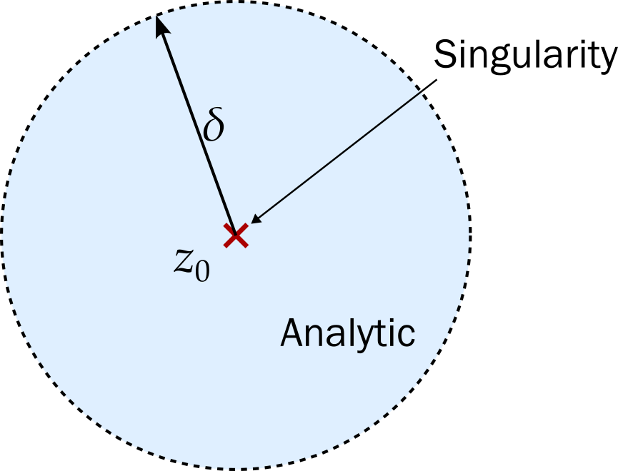
If \(f(z)\) has a singularity at \(z_0\) and there is a neighbourhood \(D\) of \(z_0\) such that \(z_0\) is the only singularity in \(D\), then \(z_0\) is an isolated singularity².

² Alternatively, if \(f\) is holomorphic in a punctured disc about \(z_0\), i.e. a disk with \(z_0\) removed, then \(z_0\) is an isolated singularity.

Figure 8.1: An isolated singularity. \(f\) is holomorphic in the blue region, except at \(z_0\) where there is a singularity. (The radius, \(\delta\), must be positive but can be arbitrarily small.)

Example 8.1 \(\displaystyle f(z) = \frac{1}{z(1 + z^2)}\) has isolated singularities at \(z = -i\), \(z = 0\) and \(z = i\).

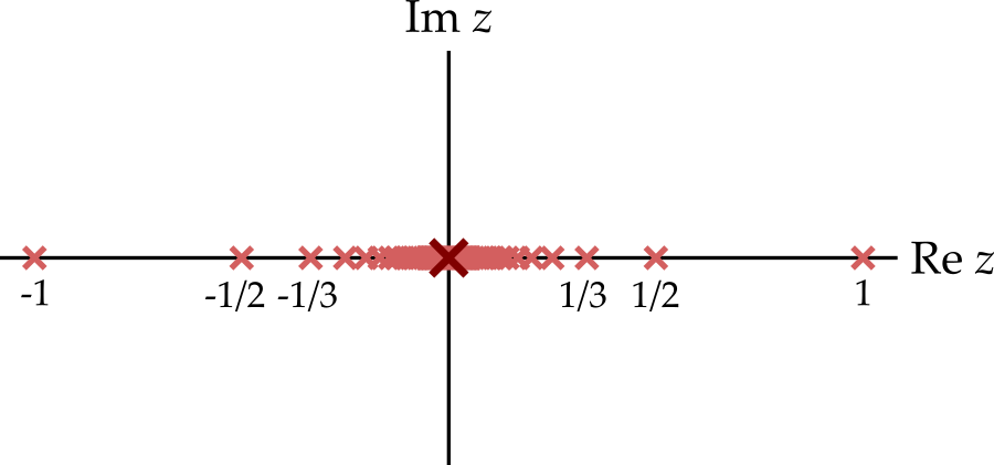
Example 8.2 Consider \(f(z) = 1 / \sin(\pi / z)\). Since \(\sin x = 0\) whenever \(x = m\pi\), for any integer \(m\), we see that \(f(z)\) must have a singularity whenever \(z = 1/m\). Each of these is isolated.

There must also be a singularity at \(z = 0\)³. However, this singularity is not isolated. No matter how small you make the radius, \(\delta\), of your disk, you will always be able to find another \(z\) within the disk where the function is singular.

³ Could we fix this like we can fix \(f(z) = (\sin z) / z\) at \(z = 0\)? No - if you consider the behaviour of \(f(z)\) you will realise that it takes a wide range of different values (indeed almost all possible values) in any disk containing \(z = 0\), no matter how small. What possible value could you assign to \(f(0)\) that would fix this?

Figure 8.2: A non-isolated singularity

Exercise

Prove the last sentence of example 8.2.

Solution

Given \(\delta > 0\), find an integer, \(m > 1/\delta\). Then the singularity at \(z = 1/m < \delta\) lies within the disk.

Notice that, according to this definition, a branch point is a non-isolated singular point, since any neighbourhood must contain points from the branch cut.

8.1.2 Poles versus essential singularities

If \(z_0\) is an isolated singularity then there is a region \(0 < \left|z - z_0\right| < \delta\) for which we have a Laurent series \[ f(z) = \sum_{n = -\infty}^\infty a_n(z - z_0)^n. \] We distinguish between the following two possibilities:

1. The Laurent series ‘truncates’ at some negative integer, i.e. there exists a positive integer \(m\) such that \(a_{-m} \neq 0\) and \(a_{n} = 0\) for all \(n < -m\). Then \[ f(z) = \frac{a_{-m}}{(z - z_0)^m} + \ldots + \frac{a_{-1}}{z - z_0} + a_0 + a_1(z - z_0) + \ldots \] and \(z_0\) is called a pole of order \(m\). A pole of order 1 is called a simple pole.
2. The Laurent series does not truncate. Then \(z_0\) is called an essential singularity.

If a function is holomorphic in a region, except for a set of poles, then the function is called meromorphic in that region.

Example 8.3 \(\displaystyle f(z) = \frac{1}{z}\) has a simple pole at \(z = 0\).

Example 8.4 \(\displaystyle f(z) = \frac{1}{(z - 1)^2}\) has a pole of order 2 at \(z = 1\).

Example 8.5 \(\displaystyle f(z) = e^{1/z} = \sum_{n = 0}^\infty \frac{z^{-n}}{n!}\), so has an essential singularity at \(z = 0\).

Example 8.6 \(\displaystyle f(z) = \frac{1}{z(1 + z^2)}\)

Here there are singularities at \(z = 0\) and \(z = \pm i\). We will find the Laurent expansion about each singularity⁴.

⁴ We will see later that this is slightly excessive.

• \(z_0 = 0\)

  In the previous lecture, we found that the Laurent expansion in the region \(0 < \left|z\right| < 1\) is \[ \frac{1}{z(1 + z^2)} = \frac{1}{z} - z + z^3 - \ldots \] and so \(z_0 = 0\) is a simple pole.

• \(z_1 = i\)

  Write \(\epsilon = z - i\) and expand in powers of \(\epsilon\). \[ \begin{aligned} f(z) &= \frac{1}{z(z + i)(z - i)}\\ &= \frac{1}{\epsilon(\epsilon + i)(\epsilon + 2i)}\\ &= \frac{1}{\epsilon}.\frac{1}{i(1 + \epsilon/i)}.\frac{1}{2i(1 + \epsilon/(2i))}\\ &= -\frac{1}{2\epsilon}\sum_{m = 0}^\infty\left(-\frac{\epsilon}{i}\right)^m\sum_{n = 0}^\infty\left(-\frac{\epsilon}{2i}\right)^n\\ &= -\frac{1}{2\epsilon}\left(1 - \frac{\epsilon}{i} + O(\epsilon^2)\right)\left(1 - \frac{\epsilon}{2i} + O(\epsilon^2)\right)\\ &= -\frac{1}{2\epsilon} + \frac{3}{4i} + O(\epsilon)\\ &= -\frac{1}{2(z - i)} + \frac{3}{4i} + O(z - i). \end{aligned} \] Hence \(z = i\) is a simple pole. A similar analysis reveals the same for \(z = -i\).

8.1.3 Removable singularities

Proceeding from non-isolated singularities to essential singularities to poles, we move from the more severe singularities to those that are easier to handle. We have not yet mentioned the simplest type of singularity to manage.

It is possible that the Laurent series has no negative powers of \(z - z_0\) at all. In this case, the singularity is said to be removable.

Example 8.7 Suppose that \[ f(z) = \begin{cases} 1 & \text{if }z = 0,\\ 0 & \text{otherwise.} \end{cases} \] The Laurent series for \(f(z)\) about \(z_0 = 0\) is just \(1\). As this contains no negative powers of \(z\), the singularity is removeable. That is, we can remove the singularity by redefining \(f(0)\) to be equal to zero.

Exercise

The function \[ f(z) = \frac{\sin z}{z} \] is undefined at \(z = 0\) and therefore has a singularity there. Classify this singularity.

Solution

We know that the Taylor series of \(\sin z\) about \(z_0 = 0\) is \[ \sin z = z - \frac{z^3}{3!} + \frac{z^5}{5!} - \ldots \] Hence the Laurent series for \(f(z)\) is \[ \frac{\sin z}{z} = 1 - \frac{z^2}{3!} + \frac{z^4}{5!} - \ldots \] Note that this series contains no negative powers of \(z\) and so the singularity is removable. If we define a new function \[ \tilde{f}(z) = \begin{cases} \frac{\sin z}{z} & \text{if } z \neq 0,\\ 1 & \text{if } z = 0 \end{cases} \] then this function is holomorphic in all of \(\mathbb{C}\).

A method for identifying a pole of \(f\) without evaluating its Laurent expansion is to analyse \[ \lim_{z \rightarrow z_0} (z - z_0)^nf(z) \] for various \(n \in \mathbb{N}\). The smallest \(n\) for which the limit exists (and is finite) gives the order of the pole⁵. If the singularity is essential, then there is no such \(n\).

⁵ One might consider that multiplying by \((z - z_0)^n\) ‘removes the pole’.

8.2 Zeros

Zeros of function \(f\) are simply points \(z = z_0\) where \(f(z_0) = 0\). Much as with singularities, we may define the order of a zero by examining the power series of the function. If the first non-zero term in the Taylor series is \(a_m(z - z_0)^m\) then we say that \(z_0\) is a zero of order \(m\). Alternatively, \(z_0\) is a zero of order \(m\) if \[ f(z_0) = f'(z_0) = \ldots = f^{(m-1)}(z_0) = 0 \] but \(f^{(m)}(z_0) \neq 0\). A zero of order \(m = 1\) is called a simple zero.

Example 8.8 \(\displaystyle f(z) = z\) has a simple zero at \(z = 0\).

Example 8.9 \(\displaystyle f(z) = (z - i)^2\) has a zero of order 2 at \(z = i\).

Example 8.10 \(\displaystyle f(z) = z^2 - 1\) has simple zeros at \(z = \pm1\). For example, around \(z = -1\) we find that the Taylor expansion is \[ -2(z + 1) + (z + 1)^2 \] and the first term is of order one.

Example 8.11 \(\displaystyle f(z) = z^2\sin z = z^3 - \frac{z^5}{3!} + \frac{z^7}{5!} - \ldots\) and so \(f\) has a zero of order 3 at \(z_0 = 0\). (It also has simple zeros at \(n\pi\) when \(n\) is a non-zero integer.)

8.3 Residue Theorem

Cauchy’s theorem has greatly simplified the calculation of integrals around closed contours, provided the integrand is holomorphic on and within the contour. Cauchy’s integral formulae can be used as tools for finding more integrals. We now wish to simplify the calculation of integrals around closed contours when the enclosed region contains isolated singularities.

8.3.1 One singularity

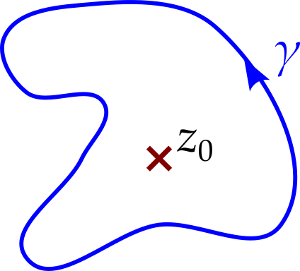
Suppose \(f(z)\) has an isolated singularity at \(z = z_0\). We can write is as a Laurent series \[ f(z) = \sum_{n = -\infty}^\infty a_n(z - z_0)^n \] valid provided \(z \neq z_0\). Consider the integral on a contour around \(z_0\).

Figure 8.3: Contour around a pole.

\[ \begin{aligned} I &= \oint_\gamma f(z)\,dz\\ &= \oint_\gamma \sum_{n = -\infty}^\infty a_n(z - z_0)^n\,dz\\ &= \sum_{n = -\infty}^\infty a_n\oint_\gamma(z - z_0)^n\,dz. \end{aligned} \] Now recall the ‘important result’, equation 6.2. This reveals that these integrals are zero, except when \(n = -1\), in which case we get \(2\pi i\). Hence \[ I = \oint_\gamma f(z)\,dz = 2\pi i a_{-1}. \tag{8.1}\] The coefficient \(a_{-1}\) is called the residue of \(f(z)\) at \(z = z_0\), also written as \(\operatorname{Res}[f(z)]_{z_0}\).

Exercise

Integrate \(\displaystyle f(z) = \frac{\cos z}{z^3}\) around the contour of figure 8.3, where \(z_0 = 0\).

Solution

The contour goes around the pole at \(z = 0\), so we will use equation 8.1. The Laurent series of \(f(z)\) is \[ \begin{aligned} \frac{\cos z}{z^3} &= \frac{1}{z^3}\left(1 - \frac{z^2}{2!} + \frac{z^4}{4!} - \ldots\right)\\ &= \frac{1}{z^3} - \frac{1}{2z} + \frac{z}{4!} - \ldots \end{aligned} \] The coefficient of \(z^{-1}\) is \(a_{-1} = -1/2\) and so \[ \int_\gamma \frac{\cos z}{z^3}\,dz = 2\pi i.\frac{-1}{2} = -\pi i. \]

8.3.2 More singularities

What happens if the contour goes around a region that contains more than one singularity? Here we will use our ability to deform contours without changing the result of the integral.

Suppose \(f(z)\) has isolated singularities at \(z_0\), \(z_1\) and \(z_2\) and we wish to calculate \[ \oint_\gamma f(z)\,dz \] on a path that encircles all of them.

Figure 8.4: Contour \(\gamma\) encircles three isolated singularities.

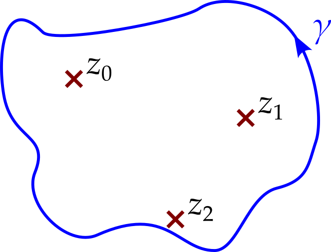
We can deform the contour, without changing the value of the integral, provided the contour does not cross a singularity. We can therefore change the contour to be as shown in figure 8.5.

Figure 8.5: The deformed contour.

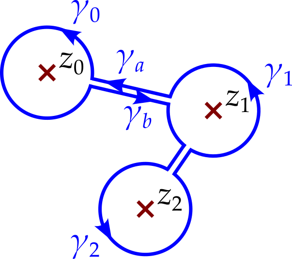
If we now take the limit of zero gap between \(\gamma_a\) and \(\gamma_b\) then the integrals along each of these contours will cancel each other. The same will also be true for the line segments between \(\gamma_1\) and \(\gamma_2\). We have now turned our integral into the sum of three integrals, each around one singularity.

Figure 8.6: Three contours.

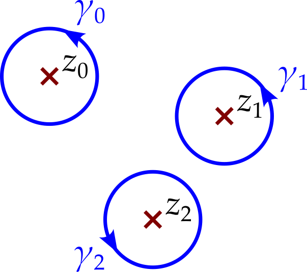
Hence \[ \oint_\gamma f(z)\,dz = \oint_{\gamma_0} f(z)\,dz + \oint_{\gamma_1} f(z)\,dz + \oint_{\gamma_2} f(z)\,dz \] and we can calculate each of these integrals using equation 8.1. The result is that \[ \begin{aligned} \oint_\gamma f(z)\,dz &= \oint_{\gamma_0} f(z)\,dz + \oint_{\gamma_1} f(z)\,dz + \oint_{\gamma_2} f(z)\,dz\\ &= 2\pi i\left(\operatorname{Res}[f]_{z_0} + \operatorname{Res}[f]_{z_1} + \operatorname{Res}[f]_{z_2}\right). \end{aligned} \]

This argument clearly generalised to any number of isolated singularities, so we get \[ \boxed { \oint_\gamma f(z)\,dz = 2\pi i\sum_k\operatorname{Res}[f]_{z_k} } \] where the \(z_k\) are each of the singularities that occur within the contour. This result is called the residue theorem.

Example 8.12 Evaluate \(\displaystyle \oint_\gamma \frac{5z - 2}{z(z - 1)}\,dz\) around the circle \(\left|z\right| = 2\), anticlockwise.

Figure 8.7: Contour and singularities

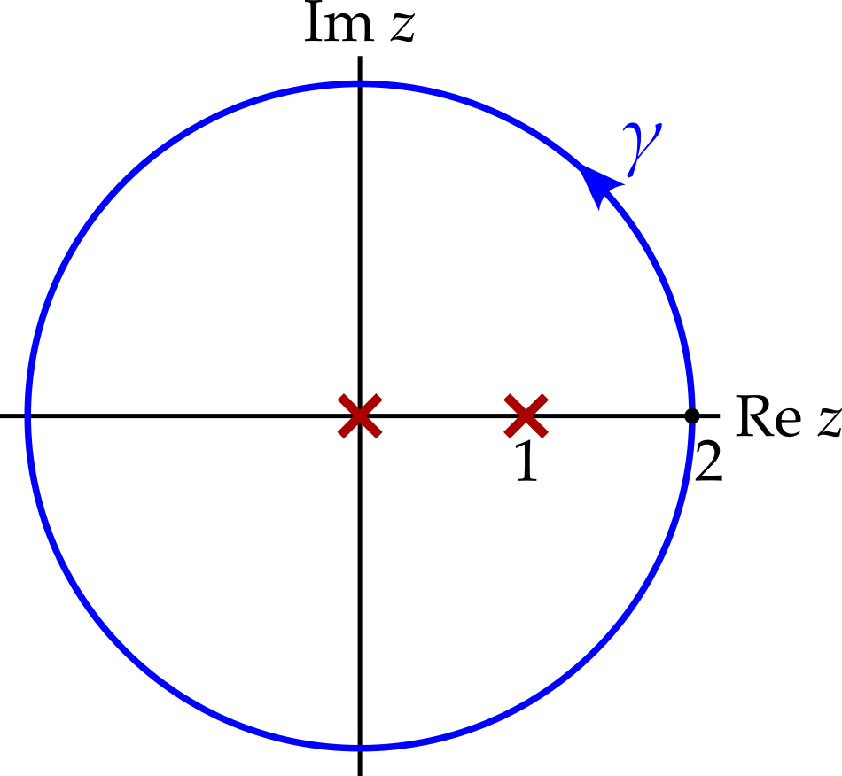
The integrand has isolated singularities at \(z = 0\) and \(z = 1\). We will need residues at both of these singularities, i.e. two Laurent expansions. Expanding around \(z = 0\), we need the Laurent series for \(0 < \left|z\right| < 1\), i.e. in the region neighbouring \(z = 0\). Similarly, when expanding around \(z = 1\), we need the Laurent series for \(0 < \left|z - 1\right| < 1\).

Expanding around \(z = 0\), we get \[ \begin{aligned} \frac{5z - 2}{z(z - 1)} &= \frac{5z - 2}{z}.\frac{-1}{1 - z}\\ &= -\frac{5z - 2}{z}\sum_{n = 0}^\infty z^n\\ &= \left(-5 - 5z - 5z^2 - \ldots\right) + \left(2z^{-1} + 2 + 2z + 2z^2 + \ldots\right)\\ &= 2z^{-1} - 3 - 3z - 3z^2 - \ldots \end{aligned} \] We therefore see that \(\operatorname{Res}[f]_0 = 2\).

To expand around \(z = 1\), we first let \(\epsilon = z - 1\) and expand in powers of \(\epsilon\). \[ \begin{aligned} \frac{5z - 2}{z(z - 1)} &= \frac{5(1 + \epsilon) - 2}{\epsilon(1 + \epsilon)}\\ &= \frac{3 + 5\epsilon}{\epsilon}.\frac{1}{1 + \epsilon}\\ &= \left(\frac{3}{\epsilon} + 5\right)(1 - \epsilon + \epsilon^2 - \ldots)\\ &= \left(\frac{3}{\epsilon} - 3 + 3\epsilon - \ldots\right) + \left(5 - 5\epsilon + 5\epsilon^2 - \ldots\right)\\ &= \frac{3}{\epsilon} + 2 - 2\epsilon + \ldots\\ &= \frac{3}{z - 1} + 2 - 2(z - 1) + \ldots \end{aligned} \] and so \(\operatorname{Res}[f]_1 = 3\). So, by the residue theorem \[ \oint_\gamma \frac{5z - 2}{z(z - 1)}\,dz = 2\pi i\left(\operatorname{Res}[f]_0 + \operatorname{Res}[f]_1\right) = 10\pi i. \]

8.4 Calculating residues

You will have realised, on working through the example above, that calculating the entire Laurent series is unnecessary when calculating residues. We need only \(a_{-1}\). Furthermore, it might not be obvious how to find the Laurent series. A formula for finding \(a_{-1}\) would be useful.

Suppose that \(f\) has a pole of finite order, \(m\), at \(z = z_0\). Then we may write \[ \begin{aligned} f(z) &= \sum_{n = -m}^\infty a_{n}(z - z_0)^n\\ &= a_{-m}(z - z_0)^{-m} + \ldots + a_{-1}(z - z_0)^{-1} + a_0 + a_1(z - z_0) + \ldots, \end{aligned} \] valid in a neighbourhood of (but not at) \(z_0\). Multiply by \((z - z_0)^m\) to get \[ (z - z_0)^mf(z) = a_{-m} + a_{-m + 1}(z - z_0) + \ldots + a_{-1}(z - z_0)^{m - 1} + \ldots \] Notice that the left hand side now has a removeable singularity at \(z = z_0\). We could define \[ g(z) = \begin{cases} (z - z_0)^mf(z) & z \neq z_0,\\ a_{-m} & z = 0. \end{cases} \] so that \(g(z)\) is holomorphic and the right hand side is its Taylor series.

Differentiate \(m - 1\) times to get \[ \frac{d^{m - 1}}{dz^{m - 1}}\left[(z - z_0)^mf(z)\right] = (m - 1)!a_{-1} + m!a_0(z - z_0) + \ldots \] It is tempting now to set \(z = z_0\), but note that, technically, the left hand side here is undefined at \(z = z_0\). So instead, take the limit as \(z\) approaches \(z_0\) and divide by \((m - 1)!\) to get \[ \boxed { \operatorname{Res}[f(z)]_{z_0} = a_{-1} = \frac{1}{(m - 1)!}\lim_{z \rightarrow z_0}\frac{d^{m - 1}}{dz^{m - 1}}\left[(z - z_0)^mf(z)\right]. } \]

Example 8.13 Returning to the previous example, consider \[ f(z) = \frac{5z - 2}{z(z - 1)}. \] At \(z = 0\) we have a simple pole, since \[ zf(z) = \frac{5z - 2}{z - 1} \] which is holomorphic at \(z = 0\). The residue is then \[ \begin{aligned} \operatorname{Res}\left[\frac{5z - 2}{z(z - 1)}\right]_{0} &= \frac{1}{0!}\lim_{z \rightarrow 0}\left[z\frac{5z - 2}{z(z - 1)}\right]\\ &= \frac{-2}{-1} = 2. \end{aligned} \]

At \(z = 1\) we have a simple pole, since \[ (z - 1)f(z) = \frac{5z - 2}{z} \] which is holomorphic at \(z = 1\). The residue is then \[ \begin{aligned} \operatorname{Res}\left[\frac{5z - 2}{z(z - 1)}\right]_{1} &= \frac{1}{0!}\lim_{z \rightarrow 0}\left[(z - 1)\frac{5z - 2}{z(z - 1)}\right]\\ &= \frac{5-2}{1} = 3. \end{aligned} \]

Hence we find the same residues as before.

Notice that, while the formula is useful for finding the residues of low order poles, it involves a lot of differentiation for higher order poles, which can get messy. In such cases, finding the Laurent expansion may be easier.