6  Complex integration

6.1 Integration with respect to a real variable

If \(f\) is a complex valued function of a real variable, \(t\), then we define \[ \int_a^b f(t)\,dt = \int_a^b \operatorname{Re}f(t)\,dt + i\int_a^b \operatorname{Im}f(t)\,dt. \] In other words, we simply integrate the real part and the imaginary part separately.

Exercise

Calculate \[ \int_0^{\pi/4}xe^{2ix}\,dx. \]

Solution

\[ \int_0^{\pi/4}xe^{2ix}\,dx = \int_0^{\pi/4}\left(x\cos2x + ix\sin2x\right)dx = \int_0^{\pi/4} x\cos2x\, dx + i\int_0^{\pi/4} x\sin2x\, dx. \] Each of these integrals can be integrated by parts to produce \[ \begin{aligned} \int_0^{\pi/4}xe^{2ix}\,dx &= \frac{1}{2}\left[x\sin2x\right]_0^{\pi/4} - \frac{1}{2}\int_0^{\pi/4}\sin2x\,dx - \frac{1}{2}i\left[x\cos2x\right]_0^{\pi/4} + \frac{1}{2}i\int_0^{\pi/4}\cos2x\,dx\\ &= \frac{1}{2}\left[x\sin2x\right]_0^{\pi/4} + \frac{1}{4}\left[\cos2x\right]_0^{\pi/4} - \frac{1}{2}i\left[x\cos2x\right]_0^{\pi/4} + \frac{1}{4}i\left[\sin2x\right]_0^{\pi/4}\\ &= \frac{\pi}{8} - \frac{1}{4} - 0 + \frac{i}{4}\\ &=\frac{\pi}{8} + \frac{1}{4}(i - 1). \end{aligned} \] Note that we could have simply calculated \[ \begin{aligned} \int xe^{2ix}\,dx &= \frac{1}{2i}xe^{2ix} - \frac{1}{2i}\int e^{2ix\,dx}\\ &= \left(\frac{1}{2i}x + \frac{1}{4}\right)e^{2ix} \end{aligned} \] and evaluated it between \(0\) and \(\pi/4\) to get \[ \int_0^{\pi/4}xe^{2ix}\,dx = \left(\frac{1}{2i}\frac{\pi}{4} + \frac{1}{4}\right)i - \frac{1}{4} = \frac{\pi}{8} + \frac{1}{4}(i - 1) \] as before.

6.2 Contour integration

What does it mean to integrate a function with respect to a complex variable? For example, let’s integrate a function \(f(z)\) from \(0\) to \(1 + i\).

First we should note that there are different ways to get from \(0\) to \(1 + i\) in the complex plane. We will need to specify the path - or contour taken.

Figure 6.1: Two paths, \(\gamma_1\) and \(\gamma_2\), from \(0\) to \(1 + i\) in the complex plane.

Hence we do not write the integral as \[ \int_0^{1 + i} f(z)\,dz \] but instead write \[ \int_{\gamma_1} f(z)\,dz \] We still need to specify the path mathematically. In the case of path \(\gamma_1\), we write \[ \gamma_1(t) = (1 + i)t, \qquad t \in [0, 1]. \] That is, as \(t\) varies from zero to one, \(\gamma_1(t)\) traces the straight-line path in the complex plane from zero to \(1 + i\). When we integrate along this path, we set \(z(t) = \gamma_1(t)\). We now convert the integral into one that is with respect to \(t\). \[ \int_{\gamma_1} f(z)\, dz = \int_0^1 f(z)\frac{dz}{dt}\,dt. \] The integration is now with respect to a real variable. This we can do! Hence this is how we define an integral with respect to a complex variable. This type of integral is referred to as a contour integral.

Let us illustrate by setting \(f(z) = \cos(z)\) and integrating along \(\gamma_1\). \[ \begin{aligned} \int_{\gamma_1} \cos z\, dz &= \int_0^1 \cos z\frac{dz}{dt}\,dt\\ &= \int_0^1 (1 + i)\cos\left((1 + i)t\right)\,dt\\ &= \bigl[\sin\left((1 + i)t\right)\bigr]_0^1\\ &= \sin(1 + i). \end{aligned} \] We could, instead, integrate along \(\gamma_2\). Notice that \(\gamma_2\) can be considered as two paths joined together, i.e. \(\gamma_3(t) = t\), where \(t\) goes from zero to one, and \(\gamma_4(t) = 1 + it\), where again, \(t\) goes from zero to one. The integral along \(\gamma_2\) is then just the sum of the integrals along \(\gamma_3\) and \(\gamma_4\). \[ \begin{aligned} \int_{\gamma_2} \cos z\, dz &= \int_{\gamma_3} \cos z\, dz + \int_{\gamma_4} \cos z\, dz\\ &= \int_0^1 \cos t\,dt + \int_0^1 i\cos(1 + it)\, dt\\ &= \bigl[\sin t\bigr]_0^1 + \bigl[\sin(1 + it)\bigr]_0^1\\ &= \sin(1) + \sin(1 + i) - \sin(1)\\ &= \sin(1 + i). \end{aligned} \] In this case, we get the same result for both paths. Is this a coincidence? We will find that it is not, but neither is it always true that integrating along different paths between the same endpoints will produce the same result.

Let us look at some more examples.

Example 6.1 Integrate \(z^2\) along half the unit circle, anticlockwise from \(z = 1\) to \(z = -1\)

The path of integration can be written as \(\gamma(t) = e^{i\pi t}\) with \(t \in [0, 1]\). Hence¹

¹ You might have noticed that the result here is exactly what one might have expected if one had written \[ \int_1^{-1}z^2\,dz = \left[\frac{z^3}{3}\right]_1^{-1} = -\frac{2}{3}, \] while the previous example is similar. However, we will soon see cases where this sort of approach no longer works.

\[ \begin{aligned} \int_\gamma z^2\,dz &= \int_0^1 \left(e^{i\pi t}\right)^2i\pi e^{i\pi t}\, dt\\ &= i\pi\int_0^1e^{3\pi it}\,dt\\ &= i\pi\left[\frac{1}{3\pi i}e^{3\pi it}\right]_0^1\\ &= \frac{1}{3}\left(e^{3\pi i} - 1\right) = -\frac{2}{3}. \end{aligned} \]

Example 6.2 Integrate \(f(z) = 1/z\) around the unit circle anticlockwise from \(z = 1\) back to \(z = 1\).

This time we write \(\gamma(t) = e^{it}\) and allow \(t\) to go from zero to \(2\pi\). We get \[ \begin{aligned} \int_\gamma \frac{1}{x}\,dx &= \int_0^{2\pi} \frac{1}{e^{it}}ie^{it}\,dt\\ &= i\int_0^{2\pi}dt = 2\pi i. \end{aligned} \]

Exercise

Integrate \(f(z) = \left|z\right|\) along each of the contours shown in figure 6.2.

Figure 6.2: Two paths, \(\gamma_1\) and \(\gamma_2\), from \(-i\) to \(i\) in the complex plane.

Solution

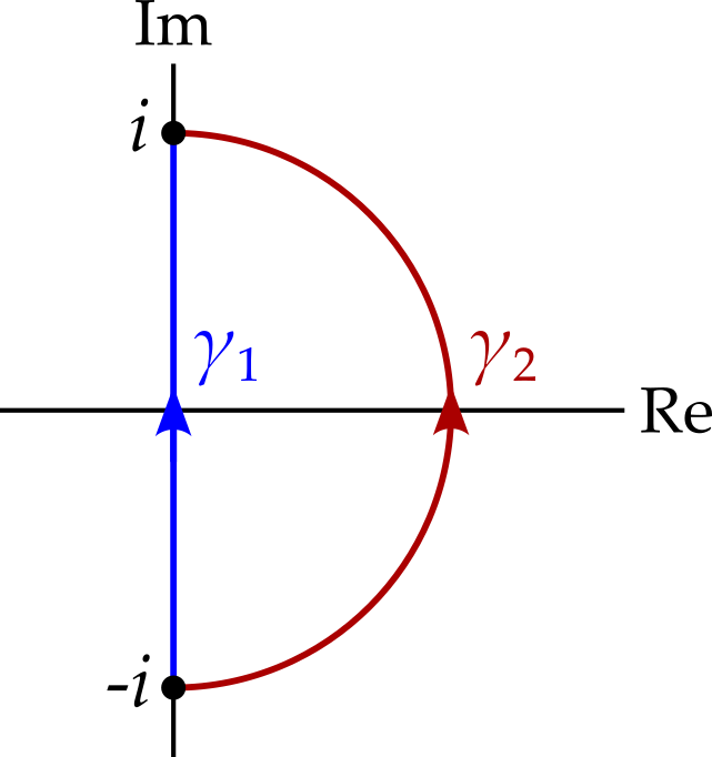
The path \(\gamma_1\) can be parameterised as \(\gamma_1(t) = it\) with \(t \in [-1, 1]\). Hence \[ \begin{aligned} \int_{\gamma_1}\left|z\right|dz &= i\int_{-1}^{1}\left|it\right|dt\\ &= i\int_{-1}^0 -t\,dt + i\int_0^1 t\,dt\\ &= i\left[-\frac{1}{2}t^2\right]_{-1}^0 + i\left[\frac{1}{2}t^2\right]_0^1\\ &= \frac{1}{2}i + \frac{1}{2}i = i. \end{aligned} \] This may at first seem surprising - the function we are integrating is real, so you might have expected a real result. However, while \(\left|z\right|\) is real, \(dz\) is not.

The alternative path can be parameterised as \(\gamma_2(t) = e^{it}\), with \(t \in [-\pi/2, \pi/2]\). Hence \[ \begin{aligned} \int_{\gamma_2}\left|z\right|dz &= \int_{-\pi/2}^{\pi/2}\left|e^{it}\right|ie^{it}\,dt\\ &= i\int_{-\pi/2}^{\pi/2}e^{it}\,dt\\ &= \bigl[e^{it}\bigr]_{-\pi/2}^{\pi/2} = 2i. \end{aligned} \] So, in this case, integrating along two different paths produces different results.

6.2.1 A useful result

Suppose the length of contour \(\gamma\) is \(\ell\) and that \(\left|f(z)\right| < f_0\) on \(\gamma\). Then \[ \begin{aligned} \left|\int_\gamma f(z)\,dz\right| &= \left|\int_0^1 (u + iv)(x' + iy')\,dt\right|\\ &\leq \int_0^1 \left|u + iv\right|.\left|x' + iy'\right|\,dt\\ &\leq \int_0^1 f_0\left|x' + iy'\right|\,dt\\ &= f_0\int_0^1 \sqrt{\left(\frac{dx}{dt}\right)^2 + \left(\frac{dy}{dt}\right)^2}\,dt\\ &= f_0\int_\gamma ds\\ &= f_0\ell. \end{aligned} \tag{6.1}\] In other words, if the modulus of the integrand is bounded above by \(f_0\), then the modulus of the integrand is bounded above by \(f_o\ell\), where \(\ell\) is the length of the contour.

6.3 Cauchy’s theorem

We are often interested in contours that are closed, i.e. that start and end at the same point so as to form a loop. When integrating around closed contours it is usually assumed, unless stated otherwise, that the contour is traversed anticlockwise.

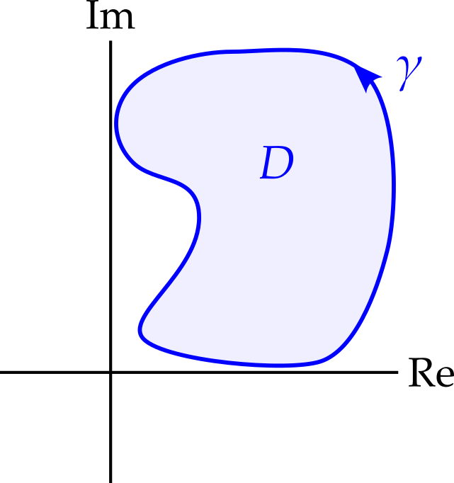
Theorem 6.1 (Cauchy’s theorem) If \(f(z)\) is holomorphic at all points on and within the closed contour \(\gamma\) then \[ \boxed { \oint_\gamma f(z)\,dz = 0. } \]

Proof. Let \(D\) be the closed region of all points on and within \(\gamma\).

Figure 6.3: The closed region \(D\) inside the contour \(\gamma\) includes all points inside on the the contour

We have \[ \begin{aligned} \oint_\gamma f(z)\,dz &= \oint_\gamma (u + iv)(dx + idy)\\ &= \oint_\gamma (u\,dx - v\,dy) + i\oint_\gamma(v\,dx + u\,dy) \end{aligned} \] where both of the integrals in the final line are real. We need to show that they both vanish, i.e. that \[ \begin{aligned} I_1 &:= \oint_\gamma(u\,dx - v\,dy) = 0,\\ I_2 &:= \oint_\gamma(v\,dx + u\,dy) = 0. \end{aligned} \]

Recall Stoke’s theorem: \[ \oint_\gamma \mathbf{F}.d\mathbf{l} = \iint_D \nabla \times \mathbf{F}.d\mathbf{a}, \] where \(\mathbf{F}\) is a vector field in three dimensions. We start by creating a two-dimensional version of Stoke’s theorem. We fix the path \(\gamma\) so that it lies in the \(x-y\) plane. We also fix \(\mathbf{F}\) so that \(F_z = 0\) and so that \(\mathbf{F}\) does not depend on \(z\). Then \(\mathbf{F}.d\mathbf{l} = F_xdx + F_ydy\) and² \[ \nabla\times\mathbf{F} = \det \begin{pmatrix} \partial_x & \partial_y & \partial_z\\ F_x & F_y & F_z\\ \hat{x} & \hat{y} & \hat{z} \end{pmatrix} = \det \begin{pmatrix} \partial_x & \partial_y & 0\\ F_x & F_y & 0\\ \hat{x} & \hat{y} & \hat{z} \end{pmatrix}. \] Hence \[ \nabla\times\mathbf{F} = (\partial_xF_y - \partial_yF_x)\hat{z}. \] Since \(d\mathbf{a}\) also points in the \(z\) direction, we get \[ \oint_\gamma (F_xdx + F_ydy) = \iint_D(\partial_xF_y - \partial_yF_x)\,dxdy. \] This is Green’s theorem. We can apply this to our line integrals. Identifying \(F_x\) with \(u\) and \(F_y\) with \(-v\), we get \[ \begin{aligned} I_1 &= \oint_\gamma(u\,dx - v\,dy)\\ &= \iint_D\left(\partial_x(-v) - \partial_yu\right)\,dxdy\\ &= -\iint_D (\partial_xv + \partial_yu)\,dxdy\\ &= -\iint_D(\partial_xv -\partial_xv)\,dxdy, \end{aligned} \] where in the last line we have used the Cauchy-Riemann equation \(\partial_yu = -\partial_vx\), which we can do since \(f = u + iv\) is holomorphic in \(D\). Hence \(I_1 = 0\).

² Here we use the shorthand \(\partial_x\) for \(\partial/\partial x\).

Moving to the second integral and identifying \(F_x\) with \(v\) and \(F_y\) with \(u\), we get \[ \begin{aligned} I_2 &= \oint_\gamma(v\,dx + u\,dy)\\ &= \iint_D (\partial_xu - \partial_yv)\,dxdy\\ &= -\iint_D(\partial_xu - \partial_xu)\,dxdy\\ &= 0 \end{aligned} \] where we have used the other Cauchy-Riemann equation, \(\partial_yv = \partial_xu\).

Hence \[ \oint_\gamma f(z)\,dz = I_1 + iI_2 = 0 \] for \(f\) holomorphic on and within \(\gamma\).

Note that there are a number of different proofs for slightly different versions of Cauchy’s theorem. For example, stronger or weaker conditions may be imposed either on the the function \(f\) or on the path \(\gamma\). For example, technically speaking, our proof requires \(f'(z)\) to be continuous, while there are versions of the proof where this is not required.

6.4 Path (in)dependence

Applying Cauchy’s theorem reveals that an integral of an entire function, between \(z_0\) and \(z_1\) does not depend on the path taken. Consider the two paths in figure 6.4.

Figure 6.4: Two paths from \(z_0\) to \(z_1\).

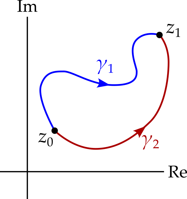
Define \[ \begin{aligned} I_1 &= \int_{\gamma_1}f(z)\,dz,\\ I_2 &= \int_{\gamma_2}f(z)\,dz. \end{aligned} \] Then \[ \begin{aligned} I_2 - I_1 &= \int_{\gamma_2}f(z)\,dz - \int_{\gamma_1}f(z)\,dz\\ &= \int_{\gamma_2}f(z)\,dz + \int_{-\gamma_1}f(z)\,dz\\ &= \int_{\gamma_2 - \gamma_1}f(z)\,dz\\ &= 0 \end{aligned} \] by Cauchy’s theorem. (Here \(-\gamma_1\) is the path \(\gamma_1\) but traversed in the reverse direction³, while \(\gamma_2 - \gamma_1\) is the path taken by following \(\gamma_2\) in the usual direction and then \(\gamma_1\) in the reverse direction.) Hence \(I_2\) = \(I_1\) - the integral (for an entire integrand) does not depend on the path - only the endpoints matter. Note that the function does not need to be entire - it need only be holomorphic on \(\gamma_1\), \(\gamma_2\) and the region between them.

³ This notation is standard but perhaps a little confusing. In particular \((-\gamma)(t)\) is not the same as \(-\gamma(t)\).

6.5 Contour deformation

We have seen that if \(f(z)\) is holomorphic on and inside a closed contour, integration becomes very easy - the answer is zero. This greatly simplifies the calculation of, for example, \[ \oint_\gamma e^{z^2}\,dz, \] when \(\gamma\) is closed. Indeed, we would not have been able to calculate this otherwise. But what if \(f(z)\) is not holomorphic inside the contour? Can Cauchy’s theorem help now?

Figure 6.5: Two closed contours in a multiply connected region, in white, where \(f(z)\) is known to be holomorphic. Can we relate the integrals of \(f\) along these two paths?

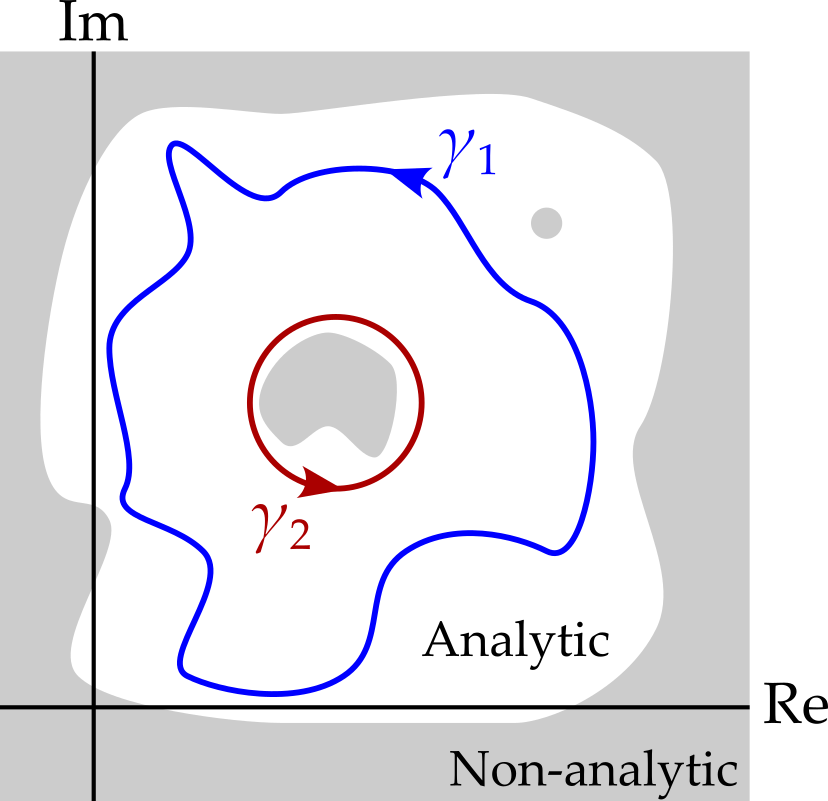
Consider figure 6.5, where the white region shows where function \(f(z)\) is holomorphic. Can we relate the integral of \(f\) on the two contours \(\gamma_1\) and \(\gamma_2\) using Cauchy’s theorem? Yes, we can. We create a new contour by creating a channel between \(\gamma_1\) and \(\gamma_2\) as shown in figure 6.6.

Figure 6.6: Two more contours are added, \(\gamma_3\) connecting \(\gamma_1\) to \(\gamma2\) and \(-\gamma_3\) going back again. Meanwhile, we now traverse \(\gamma_1\) in the reverse direction.

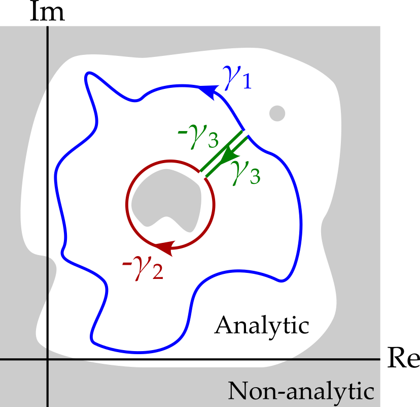
Notice that if we consider the combined path \(\gamma_1 + \gamma_3 - \gamma_2 - \gamma_3\), we see that the function is holomorphic both on and inside the contour. Hence we can evaluate the integral over the combined path in two ways. Using Cauchy’s theorem, we get \[ \oint_{\gamma_1 + \gamma_3 - \gamma_2 - \gamma_3}f(x)\,dx = 0. \] Meanwhile, \[ \begin{aligned} \oint_{\gamma_1 + \gamma_3 - \gamma_2 - \gamma_3}f(x)\,dx &= \int_{\gamma_1}f(x)\,dx + \int_{\gamma_3}f(x)\,dx + \int_{-\gamma_2}f(x)\,dx + \int_{-\gamma_3}f(x)\,dx\\ &= \int_{\gamma_1}f(x)\,dx + \int_{\gamma_3}f(x)\,dx - \int_{\gamma_2}f(x)\,dx - \int_{\gamma_3}f(x)\,dx\\ &= \int_{\gamma_1}f(x)\,dx - \int_{\gamma_2}f(x)\,dx \end{aligned} \] Comparing the two, we see that \[ \int_{\gamma_1}f(x)\,dx = \int_{\gamma_2}f(x)\,dx \]

This is useful since it means that we can take an integral along a complicated path like \(\gamma_1\) and, by deforming the contour, turn it into an integral along the much simpler circular path \(\gamma_2\). To summarise, an integral of a function over a closed path has a value that remains unchanged under a continuous deformation of the contour, provided the contour remains at all times within the region where the function is holomorphic.

6.6 An important example

An integral that will turn out to be particularly useful later is \[ \oint_\gamma (z - z_0)^n\,dz, \qquad n \in \mathbb{Z} \] where the contour, \(\gamma\), encloses the point \(z_0\). Notice that \(f(z) = (z - z_0^n)\) is holomorphic everywhere in the complex plane except potentially at \(z = z_0\).

Figure 6.7: A complicated contour around \(z_0\)

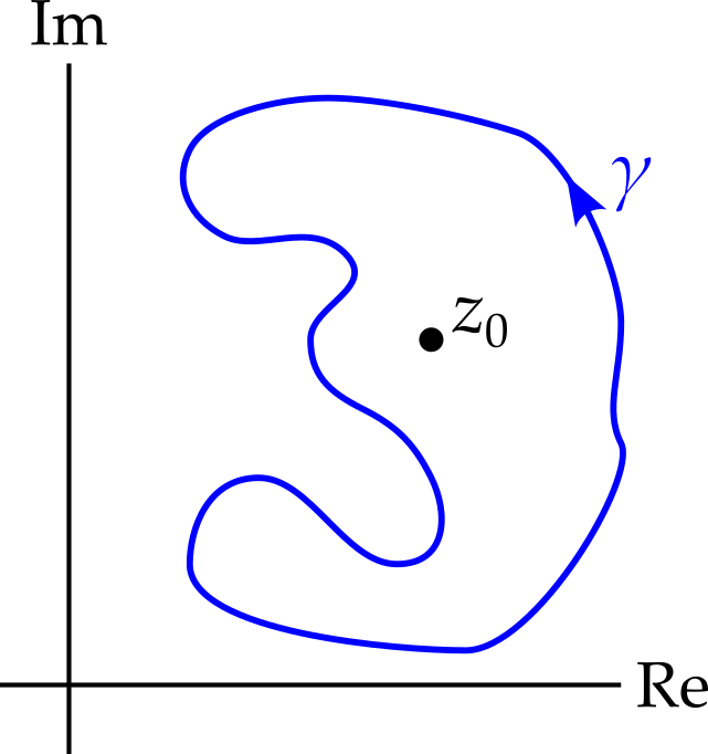
By Cauchy’s theorem, using the argument regarding contour deformation, we can continuously deform the contour until it becomes a unit circle centred at \(z_0\).

Figure 6.8: A simpler contour around \(z_0\)

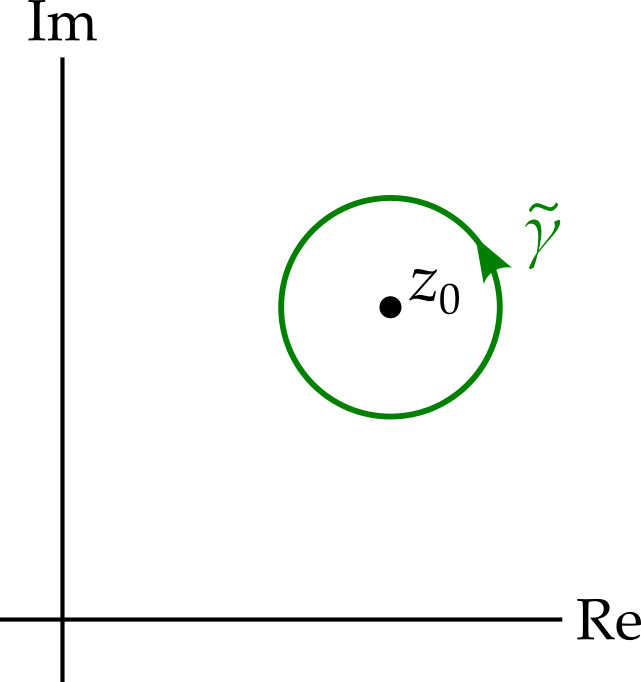
We can parameterise the path by writing \[ \widetilde{\gamma}(\theta) = z_0 + e^{i\theta}, \qquad \theta \in [0, 2\pi], \] note that \(\widetilde{\gamma}'(\theta) = ie^{i\theta}\) and then calculate our integral: \[ \begin{aligned} \oint_\gamma (z - z_0)^n\,dz &= \oint_{\widetilde{\gamma}} (z - z_0)^n\,dz\\ &= \int_0^{2\pi}e^{in\theta}.ie^{i\theta}\,d\theta\\ &= i\int_0^{2\pi}e^{i(n + 1)\theta}\,d\theta. \end{aligned} \] If \(n \neq -1\), we can continue \[ i\int_0^{2\pi}e^{i(n + 1)\theta}\,d\theta = \frac{1}{n + 1}\left[e^{i(n + 1)\theta}\right]_0^{2\pi} = 0. \] If, however, \(n = -1\), then we get \[ i\int_0^{2\pi}e^{i(n + 1)\theta}\,d\theta = i\int_0^{2\pi}1\,d\theta = 2\pi i. \] So, \[ \boxed { \oint_\gamma (z - z_0)^n\,dz = \begin{cases} 0, & \text{for } n \neq -1\\ 2\pi i, & \text{for } n = -1. \end{cases} } \tag{6.2}\] whenever the contour \(\gamma\) circles \(z = z_0\) once, anticlockwise.

Of course, for \(n \geq 0\), this result is unsurprising, since \((z - z_0)^n\) is then holomorphic everywhere, even at \(z = z_0\). The fact that, for negative \(n\), the integral is only non-zero when \(n = -1\) will prove to be most useful in what follows.