3 From real to complex analysis

In this chapter, we will explore how the basic concepts from real analysis — limits and continuity — can be extended to cover complex sequences, series and functions.

“But wait”, you say, “I haven’t studied real analysis!” Don’t worry. We will introduce these concepts for real-valued sequence and functions first, before seeing how each can be extended to the complex plane. We will also only introduce the bare essentials necessary for this course. While a thorough understanding of complex analysis would require more than this, we will attempt to reach those parts of the subject most useful to us as physicists as quickly as possible. However, we cannot avoid real analysis entirely.

Here we will discover a more precise definition of the limit than you may have seen previously, both of functions and of sequences and series. This can then be used to define what it means for a function to be continuous and will lead to definitions of differentiation and integration with which you should already be familiar.

We will also briefly look at both real and complex power series and the Taylor power series expansion of a real function. It is worth noting here that the definition of the Taylor series also works perfectly well for complex functions. However, it requires us to know how to differentiate a complex function, which is the topic of the next chapter.

3.1 Limits of sequences

3.1.1 Definition

You should already have an intuitive notion of what it means for a sequence $(a_n)_{n \in \mathbb N}$¹ (i.e. $a_1, a_2, \ldots, a_n, \ldots$) of real numbers to converge to a limit $L$. If so, you are ready for the formal definition.

¹ In this course, sequences will almost always be infinite and start with an index of 1 — in these cases, we may omit the $n \in \mathbb{N}$ part.

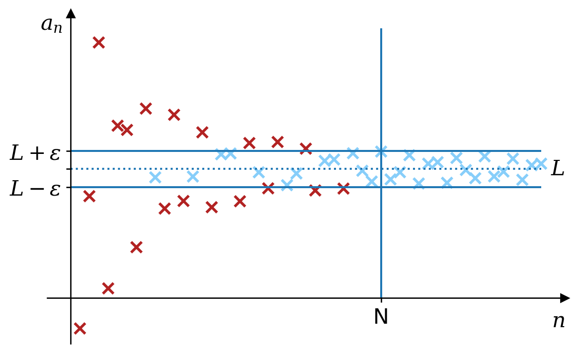
Definition 3.1 The sequence $(a_n)$ converges to the limit $L$ if, for any positive number $\epsilon$, we can find $N$ such that $n \geq N$ implies that $\left|a_n - L\right| < \epsilon$. Symbolically² \[ \forall\epsilon > 0, \exists N : n \geq N \Rightarrow \left|a_n - L\right| < \epsilon. \] Then we may write \[ \lim_{n\rightarrow\infty}a_n = L. \]

² Here I have tried to capture the essence of the definition without too many distracting details. For example, I have omitted the fact that $n$ must belong to $\mathbb{N}$.

We can think of $\epsilon$ here as being a challenge, with $N$ being the response, as follows.

“You claim that the sequence $(1/n)$ converges to zero. I challenge you to convince me that the elements of the sequence will eventually be within (and remain within) a distance of $\epsilon = 0.1$ of zero.”

“Not a problem — I choose $N = 11$. Any element of the sequence from $1/11$ onward is clearly within a distance of $0.1$ of zero.”

“Ah, but what if I challenge you to convince me that the sequence gets within $\epsilon = 0.01$ of zero.”

“Not to worry — set $N = 101$. Any element of the sequence from $1/101$ onward is within a distance of $0.01$ of epsilon.”

If you can answer any such challenge, then you have proved convergence. In this case, for any challenge, $\epsilon > 0$, we can choose $N$ to be the first integer larger than $1/\epsilon$. Then if $n \geq N$, we have $n > 1/\epsilon$ and so $\left|a_n - 0\right| = a_n = 1/n < \epsilon$.

A converging sequence of points is shown. Those points within $\epsilon$ of the limit are coloured in blue, while those further away are in red. After the $N$th element of the sequence, all points are within $\epsilon$ of the limit and are shaded in blue. — Figure 3.1: A sequence that converges to $L$. For $\epsilon > 0$ (the ‘challenge’) we can find $N$ such that, from $n = N$ onwards, all elements of the sequence lie within $\epsilon$ of the limit. Here, elements of the sequence within this range are plotted in blue. We can see that, for $n > N$, *all* points plotted are blue.

Example 3.1 We will prove that the sequence $1/2, 2/3, 3/4, 4/5, \ldots$ converges to one. In other words \[ \lim_{n \rightarrow \infty} \frac{n}{n + 1} = 1. \] Denote the $n$th term of the sequence as $a_n = n / (n + 1)$. Suppose we are given some $\epsilon > 0$. Then we can choose $N = \lceil{1 / \epsilon}\rceil$.³ Then, if $n \geq N$, we find that \[ \left|1 - a_n\right| = 1 - \frac{n}{n + 1} = \frac{1}{n + 1} < \frac{1}{N} \leq \epsilon. \] In other words, provided $n > N$, we find that $a_n$ is within $\epsilon$ of the limit $1$. Since this is true for any $\epsilon > 0$, we have shown that \[ \lim_{n \rightarrow \infty} \frac{n}{n + 1} = 1. \]

³ I.e. $1/\epsilon$ rounded up to the nearest integer, though any integer $N \geq 1/\epsilon$ would do.

3.1.2 Complex sequences

How do we change this definition of the limit to accommodate complex sequences? We don’t have to change it at all!⁴ The only difference is that the set $\{z : \left|z - L\right| < \epsilon\}$ is no longer an interval on the real line, but is a disk in the complex plane, as shown in figure 3.2.

⁴ Indeed this definition works for other mathematical objects (e.g. vectors) without modification and it requires little modification to work for any objects for which there is a well defined notion of distance.

Animation with each point of a sequence plotted in turn. The proposed limit, $L$, is shown along with a disk of radius $\epsilon$ centred on it. Any point landing in the disk is drawn in blue. Once $n > N$, all plotted points are blue and in the disk. — Figure 3.2: For complex sequences, the condition $\left|a_n - L\right| < \epsilon$ means that $a_n$ must lie in a disk of radius $\epsilon$ centred on the limit $L$. Here we see that once $n > N$, each element lands in the disk illustrated.

The analysis of the convergence of complex sequences may be simpler if we consider the sequence of real parts and the sequence of imaginary parts separately. A complex sequence converges if and only if both the real parts converge and the imaginary parts converge.

3.1.3 Cauchy’s criterion

Cauchy’s criterion for convergence states that sequence $(a_n)$ converges if and only if \[ \forall\epsilon > 0, \exists N : m, n \geq N \Rightarrow \left|a_m - a_n\right| < \epsilon. \] Notice the subtle difference between this and the definition of the limit. Here, there is no mention of the limit itself and instead of stating that the sequence elements get close to the limit, this states that the sequence elements get close to each other.

Cauchy’s criterion works for both real and complex sequences. However, this is not an obvious result.⁵ It depends on a property of the set of real numbers — completeness — that is inherited by the complex numbers. Other sets of numbers, for example the rationals, do not have this property. If we only had rational numbers, then we could find sequences satisfying Cauchy’s criterion, but without a limit.

⁵ We will not prove that Cauchy’s criterion works here.

3.2 Convergence of series

We all pronounce $\sum_{i = 0}^\infty a_i$ as “the sum from $i$ equals zero to infinity of $a_i$”. We may sometimes think of this as the sum of infinitely many numbers. However, a mathematician knows that a series is defined to be the limit of a sequence of finite sums.⁶

⁶ You should have seen examples of the dangers of thinking of a series as a simple sum. For example, given a finite sum we can always reorder the terms without changing the result. This is not always the case for infinite series.

Given the series, $\sum_{i = 0}^\infty a_i$, consider the sequence $(S_n)$ where $S_n = \sum_{i = 0}^n a_i.$ The series $\sum_{i = 0}^\infty a_i$ converges to $L$ if the sequence $(S_n)$ does.

You will already have learnt much about different types of series and how to tell whether a series is convergent or divergent in previous courses. We repeat only some key results here.

3.2.1 Absolute and conditional convergence

Definition 3.2 If $\sum_{n = 0}^\infty \left|a_n\right|$ converges then $\sum_{n = 0}^\infty a_n$ converges and is called absolutely convergent.

Absolutely convergent series are well behaved. For example, we can reorder the terms of an absolutely convergent series without worrying about changing the result.

Definition 3.3 If $\sum_{n = 0}^\infty a_n$ is convergent but not absolutely convergent then it is called conditionally convergent.

Some care needs to be taken with conditionally convergent series. In particular, reordering the terms might change the value of the sum. For example, it is known that \[ \sum_{n = 1}^\infty \frac{(-1)^{n - 1}}{n} = 1 - \frac{1}{2} + \frac{1}{3} - \frac{1}{4} + \frac{1}{5} - \ldots = \log 2. \] However, if we reorder the terms, we get \[\begin{multline*} \left(1 - \frac{1}{2} - \frac{1}{4}\right) + \left(\frac{1}{3} - \frac{1}{6} - \frac{1}{8}\right) + \left(\frac{1}{5} - \frac{1}{10} - \frac{1}{12}\right) + \ldots\\ = \left(\frac{1}{2} - \frac{1}{4}\right) + \left(\frac{1}{6} - \frac{1}{8}\right) + \left(\frac{1}{10} - \frac{1}{12}\right) + \ldots\\ = \frac{1}{2}\left(1 - \frac{1}{2} + \frac{1}{3} - \frac{1}{4} + \frac{1}{5} - \frac{1}{6} + \ldots\right) = \frac{1}{2}\log 2. \end{multline*}\]

3.2.2 Geometric series

You should already be familiar with the result \[ \sum_{n = 0}^\infty r^n = 1 + r + r^2 + \ldots = \frac{1}{1 - r},\qquad -1 < r < 1 \] for real $r$. The extension to the complex case is straightforward: \[ \sum_{n = 0}^\infty z^n = 1 + z + z^2 + \ldots = \frac{1}{1 - z},\qquad \left|z\right| < 1. \] This result is an important tool that we will use throughout the course.

3.2.3 Ratio test

The ratio test extend to complex series without modification. Recall that this states that if \[ \lim_{n \rightarrow \infty}\left|\frac{a_{n + 1}}{a_n}\right| \] is less than one, then $\sum_{n = 0}^\infty a_n$ converges absolutely. If it is greater than one, the series diverges. If it is equal to one, the test is inconclusive.

3.3 Convergence of functions

The definition of limits of functions is similar to that for sequences— indeed the limit of $f(x)$ as $x \rightarrow \infty$ is pretty much identical. However, we may also define the limit as $x$ approaches any real number.

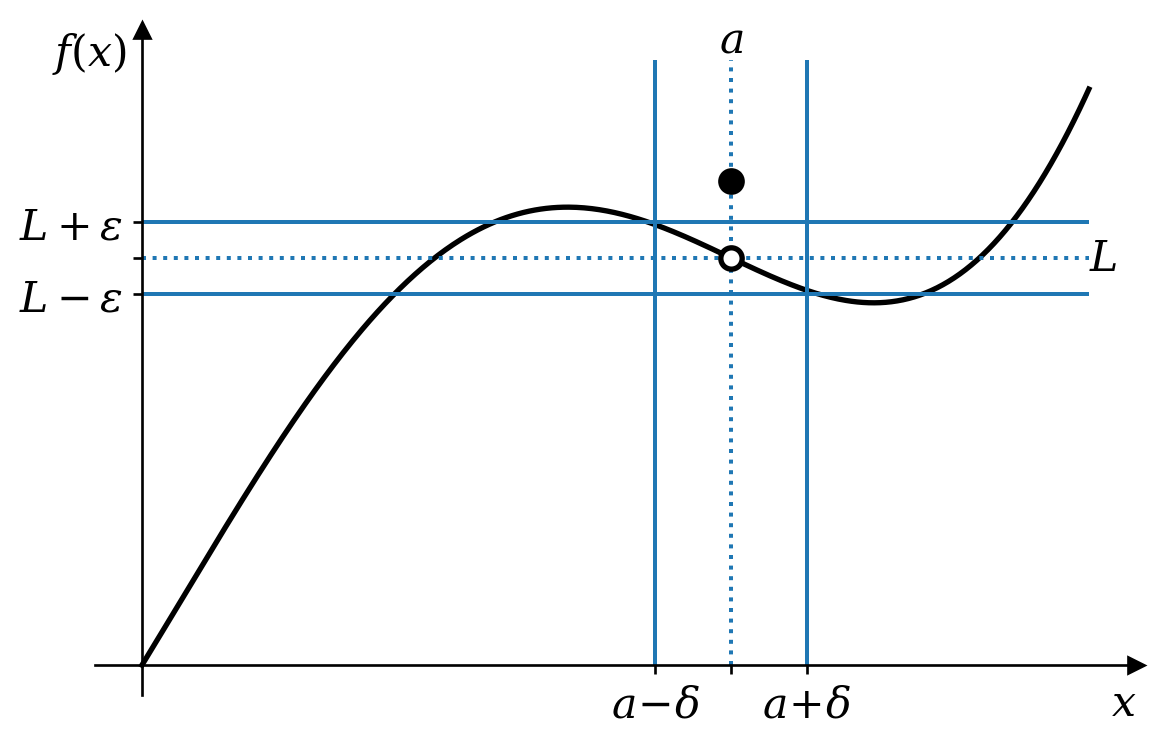
Definition 3.4 The limit of $f(x)$ at $x = a$ is $L$ if, for any positive number $\epsilon$, we can find a positive $\delta$ such that $0 < \left|x - a\right| < \delta$ implies that $\left|f(x) - L\right| < \epsilon$. Symbolically \[ \forall\epsilon > 0, \exists\delta > 0 : 0 < \left|x - a\right| < \delta \Rightarrow \left|f(x) - L\right| < \epsilon. \] Then we write \[ \lim_{x \rightarrow a}f(x) = L. \]

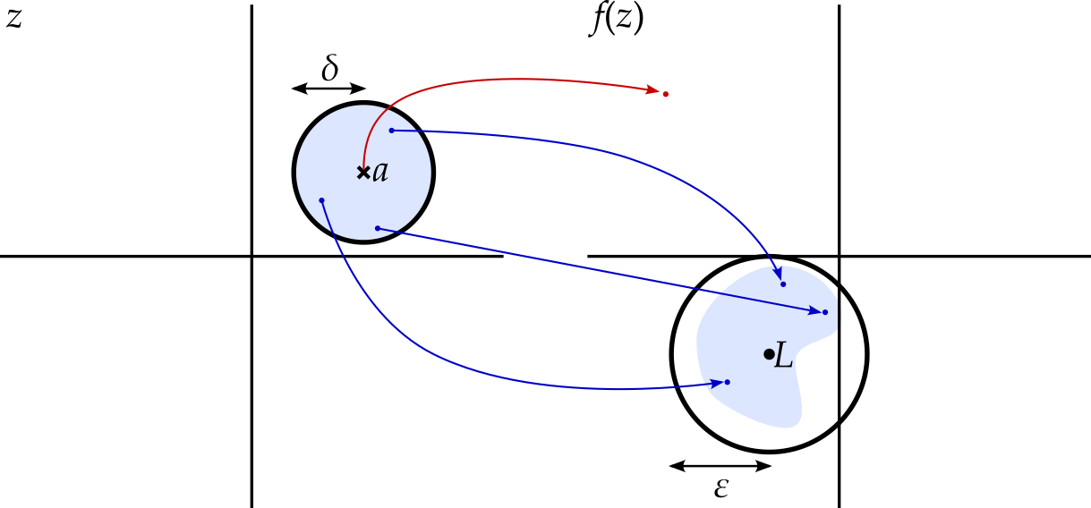
As with convergence of sequences, any $\epsilon > 0$ can be thought of as a challenge, with $\delta$ being the answer to the challenge. A single such challenge is illustrated in figure 3.3.

A function, $f$, is plotted. It is continuous everwhere, except that $f(a)$ is displaced upwards from the curve by a small distance creating a discontinuity. Ignoring this point, if we want $f(x)$ to be within $\epsilon$ of the limit $L$ at $a$, we need only ensure that $x$ is within $\delta$ of $a$. Since we can do this for any positive $\epsilon$, this confirms that $L$ is the limit of $f(x)$ as $x$ approaches $a$. — Figure 3.3: A function, $f(x)$, with $\lim_{x \rightarrow a} = L$. Given any $\epsilon > 0$ (the ‘challenge’) we can find $\delta$ such that if $x$ lies in $[a - \delta, a + \delta]$, and is *not* equal to $a$, then $f(x)$ is guaranteed to lie within $[L - \epsilon, L + \epsilon]$. The limit does not depend on the value of $f(a)$ itself, which may be different to the limit or may be undefined.

There are a few important features of this definition:

The restriction that $\left|x - a\right| > 0$ means that $f(a)$ need not equal $L$ or be within $\epsilon$ of $L$.
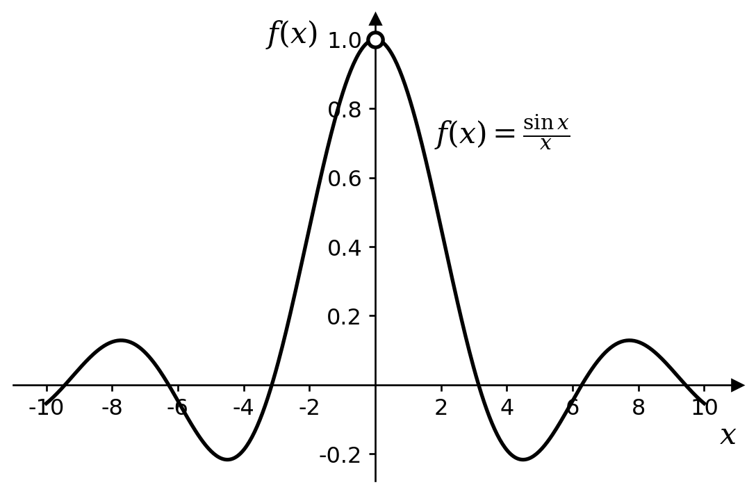
Indeed, $f(a)$ need not even be defined. For example, if $f(x) = (\sin x) / x$ then $f(0)$ is not defined, but we can still claim that $\lim_{x \rightarrow 0}f(x) = 1$. (See figure 3.4.)
We require $f(x)$ to be close to $L$ for all $x$ close enough to $a$, regardless of whether $x < a$ or $x > a$. In other words, the limit should be the same whether $x$ approaches $a$ from above or below.

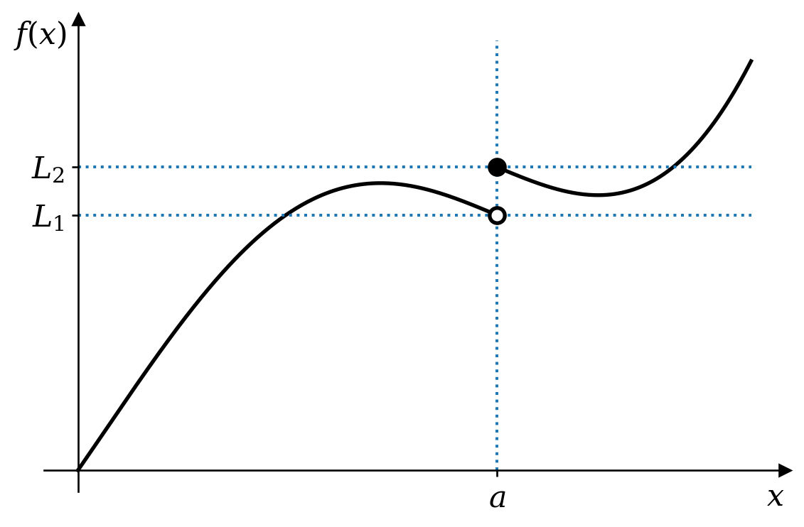
The graph is like a simple sine wave, except that the amplitude of the wave goes like $1/x$. This function is undefined at $x = 0$, since we get zero divided by zero. However, as $x$ approaches zero, $1/x$ becomes very large but $\sin x$ becomes small. Multiplying these together, we get a value that approaches one as $x$ approaches zero. — Figure 3.4: Graph of the function $f(x) = (\sin x) / x$. Note that this is not defined at $x = 0$ but has a well defined limit there.

We can define one-sided limits. The left limit \[ \lim_{x \rightarrow a^-}f(x) \] considers $x$ approaching $a$ from the left; that is we only consider values of $x$ less than $a$. The right limit \[ \lim_{x \rightarrow a^+}f(x) \] considers $x$ approaching $a$ from the right. These can be different as illustrated in figure 3.5. The limit $\lim_{x \rightarrow a}f(x)$ exists only if the left and right limits are equal.

A graph of a function that is continuous, except for a jump at $x = a$ where the value increases suddenly. — Figure 3.5: A function, $f(x)$, with different left and right limits at $x = a$. Here $\lim_{x \rightarrow a^-}f(x) = L_1$ while $\lim_{x \rightarrow a^+}f(x) = L_2$. The (standard) limit, $\lim_{x \rightarrow a}f(x)$ does not exist because the left and right limits do not agree. (The solid circle indicates that $f(a) = L_2$, while the hollow circle indicates a point *not* on the graph.)

Exercise

How might the symbolic definition of the limit be adapted to create definitions of the left and right limits?

Solution

The left limit of $f(x)$ at $x = a$ is $L$ if \[ \forall\epsilon > 0, \exists\delta > 0 : 0 < a - x < \delta \Rightarrow \left|f(x) - L\right| < \epsilon. \] Similarly, the right limit of $f(x)$ at $x = a$ is $L$ if \[ \forall\epsilon > 0, \exists\delta > 0 : 0 < x - a < \delta \Rightarrow \left|f(x) - L\right| < \epsilon. \]

The notion of approaching $x$ from different directions will become even more important when we extend this to complex functions.

3.3.1 Complex functions

As with complex sequences, the definition of the limit of a function needs no change as we move from real functions to complex functions, but sets that were intervals on the real line become disks in the complex plane. Here $\left|f(z) - L\right| < \epsilon$ defines a disk in the Argand diagram for $f(z)$, while $0 < \left|z - a\right| < \delta$ defines a punctured disk - a disk with the centre point removed - in the complex plane of $z$.

A disk of radius $\delta$ around $z = a$ and shaded in blue is mapped into a blue region within the disk of radius $\epsilon$ around the limit $L$. A red arrow indicates that $a$ need not be mapped into the disk and that $f(a)$ does not affect the limit. — Figure 3.6: Finding a disk around $z = a$ small enough to ensure that all points in the disk (with the possible exception of $a$ itself) map into a disk of radius $\epsilon$ around the limit $L$. The value of $f(a)$ need not lie in the disk and is irrelevant to the definition of the limit.

3.4 Continuity

Having defined limits of functions, the definition of continuity is straightforward.

Definition 3.5 A function $f$ is continuous at $a$ if $f(a) = \lim_{x \rightarrow a}f(x)$.

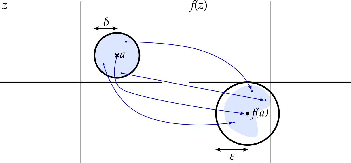
Inserting the definition of the limit, we find that $f(x)$ is continuous at $x = a$ if, for any positive number $\epsilon$, we can find a positive $\delta$ such that $\left|x - a\right| < \delta$ implies that $\left|f(x) - f(a)\right| < \epsilon$, or symbolically \[ \forall\epsilon > 0, \exists\delta > 0 : \left|x - a\right| < \delta \Rightarrow \left|f(x) - f(a)\right| < \epsilon. \] This captures the notion that, given a continuous function, it is possible to make the change, $f(x + h) - f(x)$, in the function as small as we like, provided we ensure that the step size, $h$, is small.

Again, the definition of continuity requires no adjustment in order to work for complex functions too.

A disk of radius $\delta$ around $z = a$ and shaded in blue is mapped into a blue region within the disk of radius $\epsilon$ around the limit $L$. — Figure 3.7: To guarantee that the change in $f(z)$ is small ($< \epsilon$), just ensure that you make a small enough change in $z$ ($< \delta$).

3.5 Power series

3.5.1 Real power series

A real power series is a series of the form \[ P(x) = \sum_{n = 0}^\infty a_nx^n \] where each of the coefficients $a_n$ are real numbers.

Before we extend this to complex power series, let’s examine for which $x$ the series converges. Using the ratio test, we calculate the ratio \[ \lim_{n \rightarrow \infty}\left|\frac{a_{n + 1}x^{n + 1}}{a_nx^n}\right| = \left|x\right|\lim_{n \rightarrow \infty}\left|\frac{a_{n + 1}}{a_n}\right|. \] We require this ratio to be less than one in order to guarantee convergence. Let \[ L = \lim_{n \rightarrow \infty}\left|\frac{a_{n + 1}}{a_n}\right|. \] If $L = 0$ then the series converges for any value of $x$. If $L$ is infinite then the series diverges for any value of $x$ except zero. Otherwise we let $r = 1 / L$ and note that we require \[ \frac{\left|x\right|}{r} < 1, \] i.e. $-r < x < r$. This range of values for which the series converges is known as the interval of convergence. If $\left|x\right| > r$ then the series diverges, while the test is inconclusive for $x = \pm r$.

3.5.2 Complex power series

The extension to complex power series is straightforward. A complex power series is a series of the form⁷ \[ P(z) = \sum_{n = 0}^\infty a_nz^n \] where each of the coefficients $a_n$ are complex numbers.

⁷ You will have noticed that while a real variable is often called $x$, we tend to use $z$ for a complex variable. This is just a commonly used convention — we can of course use any letter we wish.

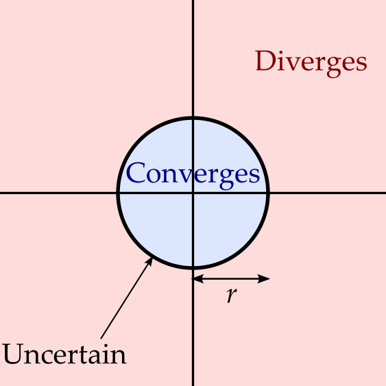
The ratio test analysis proceeds as before, giving us \[ \frac{\left|z\right|}{r} < 1 \] but now this becomes $\left|z\right| < r$ and we have a disk of values for $z$ for which the series converges. The radius, $r$, of this disk is called the radius of convergence.

A disk of radius $r$ around $z = 0$ is plotted to illustrate the radius of convergence. A pale blue is used within the disk, to indicate convergence, while a pale pink is used outside to indicate divergence. — Figure 3.8: Within the radius of convergence (where $\left|z\right| < r$), a power series converges. Outside the radius of convergence ($\left|z\right| > r$) a power series diverges. For points on the radius of convergence ($\left|z\right| = r$) the situation is uncertain — the series may converge for some $z$ but not others.

3.5.3 Taylor series

Taylor expansions are a way of expressing a function as an infinite power series. While this idea extends seamlessly to complex functions, it requires us to be able to differentiate complex functions — the topic of the next chapter. Here, therefore, we will deal only with real functions, but note that the same idea will work for complex functions once we know how to differentiate them.

Let’s assume that our function $f(x)$ can be differentiated as often as we like and that it can be written as a power series in $(x - x_0)$, i.e. \[ f(x) = \sum_{n = 0}^\infty a_n(x - x_0)^n = a_0 + a_1(x - x_0) + a_2(x - x_0)^2 + \ldots \tag{3.1}\] Let’s find the coefficients $a_n$.

Set $x = x_0$. Then equation 3.1 becomes $f(x_0) = a_0$.
Differentiate equation 3.1 to get \[ f'(x) = a_1 + 2a_2(x - x_0) + 3a_3(x - x_0)^2 + \ldots \] Setting $x = x_0$ now gives $f'(x_0) = a_1$.
Differentiate again to get \[ f''(x) = 2a_2 + 6a_3(x - x_0) + 12a_4(x - x_0)^2 + \ldots \] Setting $x = x_0$ gives $f''(x_0) = 2a_2$.
Shall we differentiate again? Why not! \[ f^{(3)}(x) = 6a_3 + 24a_4(x - x_0) + 60a_4(x - x_0)^2 + \ldots \] and setting $x = x_0$ gives us $f^{(3)}(x_0) = 6a_3$.

Repeating, we get \[ f^{(n)}(x_0) = n!a_n \] which we rearrange to get \[ a_n = \frac{f^{(n)}(x_0)}{n!}. \] Hence, provided such a power series expansion exists, the Taylor series for $f(x)$ around $x = x_0$ is given by \[ \boxed { f(x) = \sum_{n = 0}^\infty \frac{f^{(n)}(x_0)}{n!}(x - x_0)^n. } \] A function $f(x)$ is called analytic at $x_0$ if its Taylor series around $x_0$ exists and converges to $f(x)$ in some neighbourhood of $x_0$.

Example 3.2 Let us find the Taylor series for $f(x) = e^x$ around $x_0 = 0$. Notice that $f'(x) = e^x$, $f''(x) = e^x$, etc., so $f(0) = f'(0) = f''(0) = \ldots = 1$. Hence $a_n = 1 / n!$ and we get \[ f(x) = e^x = \sum_{n = 0}^\infty \frac{x^n}{n!}, \] which I hope you recognize as the correct power series expansion of $e^x$.

We can now find the interval of convergence. The ratio test indicates that the series converges whenever \[ \left|x\right|\lim_{n \rightarrow \infty}\left|\frac{a_{n + 1}}{a_n}\right| < 1 \] Now \[ \left|\frac{a_{n + 1}}{a_n}\right| = \frac{n!}{(n + 1)!} = \frac{1}{n + 1}, \] so \[ \lim_{n \rightarrow \infty}\left|\frac{a_{n + 1}}{a_n}\right| = 0. \] Hence the series converges for all $x$

Example 3.3 Now let us find the Taylor series of $f(x) = 1 / (1 - x)$ around the point $x_0 = 0$. Start by noticing that $f(0) = 1$. Now differentiate to find that

$f'(x) = \frac{1}{(1 - x)^2}$, so that $f'(0) = 1$,
$f''(x) = \frac{2}{(1 - x)^3}$, so that $f''(0) = 2$,
$f^{(3)}(x) = \frac{6}{(1 - x)^4}$, so that $f^{(3)}(0) = 6$,
…
$f^{(n)}(x) = \frac{n!}{(1 - x)^(n + 1)}$, so that $f^{(n)}(0) = n!$

We therefore find that \[ a_n = \frac{f^{(n)}(0)}{n!} = \frac{n!}{n!} = 1 \] for all values of $n$. Hence \[ f(x) = \frac{1}{1 - x} = 1 + x + x^2 + x^3 + ... \] We could, of course, have worked this out more simply by recognizing the formula for geometric series that we found earlier.

To work out the interval of convergence, we simply find \[ \lim_{n \rightarrow \infty}\left|\frac{x^{n + 1}}{x^n}\right| = \left|x\right| \] and so the series converges whenever $\left|x\right| < 1$