9  Real Integrals

9.1 The uniqueness theorem and analytic continuation

We will soon be applying what we have learned to the calculation of real integrals, but before we do, it will be useful to briefly consider the topic of analytic continuation.

Suppose we have a well-behaved function \(f\) defined on a small subset, \(S\), of the complex plane. We wish to extend its domain by finding a function \(g\) that agrees with \(f\) in subset \(S\) and is holomorphic in a larger region, \(R\), containing \(S\). The function \(g\) is an analytic continuation of \(f\).

Figure 9.1: \(f\) is defined in region \(S\). If \(g\) is holomorphic in larger region \(R\) and \(f(z) = g(z)\) for \(z \in S\) then it is an analytic continuation of \(f\).

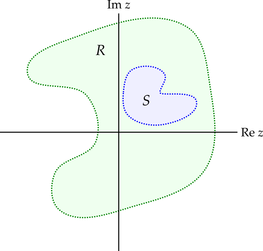
Theorem 9.1 (Uniqueness) Let \(f\) and \(g\) be holomorphic functions in region \(R\) and let \(S\) be a subset of \(R\). If \(f(z) = g(z)\) for all \(z \in S\) then \(f = g\) in region \(R\), provided the set \(S\) has a limit point in \(R\).

Proof. Omitted.

What is a limit point? Rather than explain this detail, let’s give some examples of suitable sets \(S\). If \(S\) is a disk, or contains a disk, no matter how small, then the theorem will work¹. Alternatively, if \(S\) is a line segment, or contains a line segment, no matter how short, the theorem will still work². In particular, \(S\) can be the real axis, or just a segment of the real axis.

¹ I.e. \(S\) will ‘have a limit point in \(R\)’.

² However, if \(S\) is just a set of isolated points, then the theorem does not work.

The uniqueness theorem tells us that analytic continuations, if they exist, must be unique. Suppose \(f\) is holomorphic in region \(S\) and that \(g\) and \(h\) are both analytic continuations to larger region \(R\). Since \(g\) and \(h\) are both holomorphic on \(R\) and agree on \(S\), we must have \(g = h\), by the uniqueness theorem.

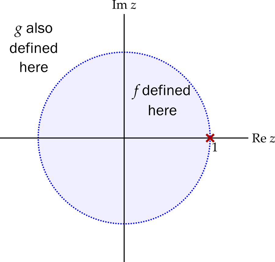
Example 9.1 Let \[ f(z) = \sum_{n = 0}^\infty z^n \quad \text{ and } \quad g(z) = 1/(1 - z). \] Function \(g\) is defined and holomorphic across the entire complex plane, except at \(z = 1\). Function \(f\), however, is only defined within the radius of convergence, i.e. in the unit circle centred at \(z = 0\), where it is holomorphic and agrees with \(g\). Therefore \(g\) is an analytic continuation of \(f\) to the region \(\mathbb{C}\setminus\{1\}\).

Figure 9.2: While \(f = \sum_{n = 0}^\infty\) is defined and holomorphic only in the shaded region, \(g = 1 / (1 - z)\) analytically extends \(f\) to the whole of \(\mathbb{C}\), with the exception of \(z = 1\).

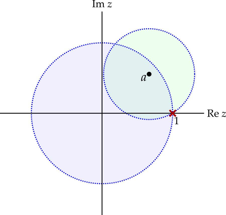
In this example, finding an analytic continuation was straightforward, but what about more challenging cases? One strategy is to Taylor expand \(f\) about a point in the region and to analyse the resulting radius of convergence. While certainly not guaranteed, it is possible that the resulting disk will extend out of the domain on which the function is originally defined.

Figure 9.3: Taylor expanding about \(z = a\) produces a sufficiently large radius of convergence to analyticall continue function \(f\) into a new region.

It is worth mentioning that you have already seen many examples of analytic continuation. For example, the complex exponential, \(f(z) = e^z\), and the complex cosine, \(f(z) = \cos z\), that we defined so carefully at the beginning of the course are analytic continuations of their real counterparts. The uniqueness theorem now tells us that this was essentially the only way that these functions could be extended to cover the complex plan. Any other methods of defining \(e^z\) would either produce exactly the same function, or fail to produce a holomorphic function.

In what follows, we will analytically continue many other functions from \(\mathbb{R}\) to \(\mathbb{C}\)³. In practice, having already handled the basic functions, this will merely involve replacing \(x\) with \(z\). This will be done as part of a process for converting real integrals into integrals along closed paths in the complex plane, so as to exploit the complex analysis tools we have recently learned.

³ Or to much of \(\mathbb{C}\)

9.2 Real integrals

Suppose we wish to use complex analysis techniques to calculate a real integral \[ I = \int_a^b f(x)\,dx. \] There are a number of methods to do this and sometimes some ingenuity is required to find a suitable contour of integration. We will examine two broad strategies.

1. Change variables, from \(x\) to a complex variable \(z\) that follows a convenient closed contour in the complex plane as \(x\) goes from \(a\) to \(b\).
2. Analytically continue the integrand so that it is defined on the complex plane, with the contour lying between \(a\) and \(b\) on the real axis. Then close the contour in a way that ensures that the integral along the new segments of the contour are either easy to calculate or related, in some simple way, to \(I\).

Both approaches are then concluded by using the residue theorem (or Cauchy’ theorem) to calculate the contour integral and thus find \(I\). We will illustrate these methods with some examples.

9.3 Trigonometric integrals

Here we consider integrals of the form \[ I = \int_0^{2\pi} f(\sin\theta, \cos\theta)\,d\theta, \] where \(f\) is finite and single-valued for all \(\theta\). Make a change of variable to \(z = e^{i\theta}\). Notice how this turns the real integral into a complex one around a closed contour - as \(\theta\) goes from \(0\) to \(2\pi\), \(z\) travels around the unit circle around \(z = 0\).

We need to write \(d\theta\) in terms of our new variable \(z\): \[ dz = ie^{i\theta}\,d\theta \quad \Rightarrow \quad d\theta = -i\frac{dz}{z} \] We will also need to write the integrand in terms of \(z\), so we note that \[ \cos\theta = \frac{e^{i\theta} + e^{-i\theta}}{2} = \frac{1}{2}(z + z^{-1}) \] and \[ \sin\theta = \frac{e^{i\theta} - e^{-i\theta}}{2i} = \frac{1}{2i}(z - z^{-1}). \] If \(f\) also includes \(\cos(n\theta)\) or \(\sin(n\theta)\), for some \(n\), then we can use \[ \cos(n\theta) = \frac{1}{2}(z^n + z^{-n}),\qquad \sin(n\theta) = \frac{1}{2i}(z^n - z^{-n}). \] Performing the change of variables, we get \[ I = -i\oint_\gamma f\left(\frac{1}{2i}(z - z^{-1}), \frac{1}{2}(z + z^{-1})\right)\,\frac{dz}{z}, \] where \(\gamma\) is the unit circle. We can now use the residue theorem to complete the calculation.

Example 9.2 \[ I = \int_0^{2\pi}\frac{1}{2 - \cos\theta}\,d\theta. \] Start by noticing that \(2 - \cos\theta\) is never zero on the real line, so the integrand has no singularities in \([0, 2\pi)\). Applying the substitution \(z = e^{i\theta}\), we get \[ \begin{aligned} I &= -i\oint_\gamma \frac{1}{2 - \frac{1}{2}(z + z^{-1})}\,\frac{dz}{z}\\ &= -i\oint_\gamma \frac{1}{2z - \frac{1}{2}z^2 - \frac{1}{2}}\,dz\\ &= 2i\oint_\gamma \frac{1}{z^2 - 4z + 1}\,dz. \end{aligned} \] The integrand has poles when the denominator is zero, i.e. when \(z = 2 \pm \sqrt{3}\). It will be convenient to define \[ \begin{aligned} z_+ &= 2 + \sqrt{3},\\ z_- &= 2 - \sqrt{3}. \end{aligned} \] Now notice that only one of these poles will contribution to the integral, because only one is inside the contour.

Figure 9.4: Location of the poles relative to the contour. Only the residue at \(z = 2 - \sqrt{3}\) contributes to the integral. (Not to scale.)

Factorising the denominator, we therefore have \[ \oint_\gamma \frac{1}{z^2 - 4z + 1}\,dz = 2\pi i\operatorname{Res}\left[\frac{1}{(z - z_+)(z - z_-)}\right]_{z_-}. \] The pole at \(z_-\) is a simple pole, so we have \[ \begin{aligned} \operatorname{Res}\left[\frac{1}{(z - z_+)(z - z_-)}\right]_{z_-} &= \lim_{z \rightarrow z_-}\frac{z - z_-}{(z - z_+)(z - z_-)}\\ &= \frac{1}{z_- - z_+} = -\frac{1}{2\sqrt{3}}. \end{aligned} \] Putting this all together, we get \[ I = 2i \times 2\pi i \times -\frac{2}{2\sqrt{3}} = \frac{2\pi}{\sqrt{3}}. \]

Example 9.3 \[ I = \int_0^{2\pi} \frac{\cos2\theta}{5 - 4\cos\theta}\,d\theta. \] Perform the substitution \(z = e^{i\theta}\) to get \[ \begin{aligned} I &= -i\oint_\gamma\frac{\frac{1}{2}(z^2 + z^{-2})}{5 - 2(z + z^{-1})}\,\frac{dz}{z}\\ &= \frac{i}{4}\oint_\gamma \frac{z^4 + 1}{z^2(z - \frac{1}{2})(z - 2)}\,dz. \end{aligned} \]

Figure 9.5: Location of the poles relative to the contour. Here residues must be calculated at \(z = 0\) and \(z = 1/2\).

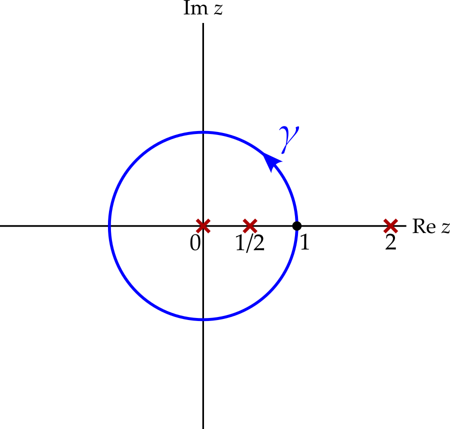
The integrand has a pole of order 2 at \(z = 0\) and simple poles at \(z = 1/2\) and \(z = 2\). Only the first two poles contribute, since the third lies outside the contour \(\gamma\).

The residue at \(z = 0\) is \[ \begin{aligned} \operatorname{Res}&\left[\frac{z^4 + 1}{z^2(z - \frac{1}{2}(z - 2))}\right]_0 = \frac{1}{1!}\lim_{z \rightarrow 0}\left[\frac{d}{dz}\frac{z^4 + 1}{(z - \frac{1}{2})(z - 2)}\right]\\ &\qquad= \lim_{z \rightarrow 0}\left[\frac{4z^3(z - \frac{1}{2})(z - 2) - (z^4 + 1)\left((z - \frac{1}{2}) + (z - 2)\right)}{\left((z - \frac{1}{2})(z - 2)\right)^2}\right]\\ &\qquad= \frac{5}{2}. \end{aligned} \] The residue at \(z = 1/2\) is somewhat easier to calculate - it is \[ \begin{aligned} \operatorname{Res}\left[\frac{z^4 + 1}{z^2(z - \frac{1}{2})(z - 2))}\right]_{1/2} &= \lim_{z \rightarrow 1/2}\left[\frac{z^4 + 1}{z^2(z - 2)}\right]\\ &= \frac{17/16}{-3/8}\\ &= -\frac{17}{6}. \end{aligned} \] We therefore get \[ I = \frac{i}{4} \times 2\pi i \times \left(\frac{5}{2} - \frac{17}{6}\right) = \frac{\pi}{6}. \]

9.4 Infinite integrals

For trigonometric integrals, we chose the first strategy - change of variables. For infinite integrals, i.e. \[ I = \int_{-\infty}^\infty f(x)\,dx, \] we will use the second strategy - closing the contour.

We assume that

• f(z) is holomorphic in the upper half-plane (\(\operatorname{Im}z \geq 0\)), except for a finite number of isolated singularities.
• In the \(\left|z\right| \rightarrow \infty\) limit in the upper half-plane, \(f(z)\) approaches zero faster than \(1/z\), i.e. \[ \lim_{\left|z\right| \rightarrow \infty}zf(z) \rightarrow 0. \]

Consider what happens if we integrate \(f(z)\) on the contour shown in figure 9.6.

Figure 9.6: Completing the contour in the upper half plane.

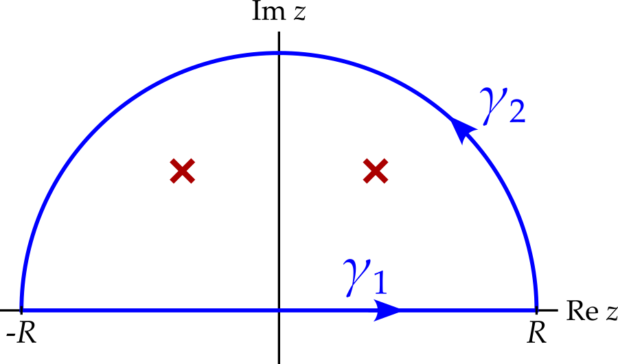
On \(\gamma_1\), \(z\) is real and hence \[ \int_{\gamma_1}f(z)\,dz = \int_{-R}^R f(x)\,dx. \] Taking the limit as \(R\) approaches infinity, we have \[ \lim_{R \rightarrow \infty}\int_{\gamma_1}f(z)\,dz = \int_{-\infty}^\infty f(x)\,dx = I, \] which is the integral we are trying to find.

It would be convenient if the integral along \(\gamma_2\) approached zero as \(R\) tends to infinity. Recall the ‘useful result’ from section 6.2.1: \[ \left|\int_\gamma f(z)\,dz\right| \leq f_0\ell, \] where \(\ell\) is the length of the contour and \(f_0\) is an upper bound on \(\left|f(z)\right|\), i.e. \(\left|f(z)\right| \leq f_0\) on \(\gamma\). The length of the contour is \(\ell = \pi R\), while for \(f_0\) we can choose the maximum value⁴ of \(f(z)\) on contour \(\gamma_2\) - call this \(f_{\text{max}}(R)\). Then we have \[ \left|\int_{\gamma_1} f(z)\,dz\right| \leq \pi Rf_{\text{max}}(R). \] But we are told that \(zf(z)\) approaches zero as \(R\) gets large, which means that \(Rf_{\text{max}}(R)\) must too. Hence \[ \lim_{R \rightarrow \infty}\int_{\gamma_2}f(z)\,dz = 0. \]

⁴ There is a small technical issue here - does this maximum exist?

This means that, to find \(I\) we must calculate the integral around the closed contour, which we can do by using the residue theorem.

Example 9.4 \[ I = \int_0^\infty \frac{1}{x^2 + 1}\,dx. \] Observe that the integrand here is an even function⁵, i.e. \(f(x) = f(-x)\), and so \[ I = \frac{1}{2}\int_{-\infty}^\infty \frac{1}{x^2 + 1}\,dx. \] We now consider the analytic continuation of the integrand, \[ f(z) = \frac{1}{z^2 + 1} = \frac{1}{(z - i)(z + i)} \] and integrate along the contour in figure 9.7.

⁵ Integrals are not always immediately suitable for solving using complex analysis - some work using other techniques may be required to get an integral into the correct form.

Figure 9.7: Completing the contour in the upper half plane.

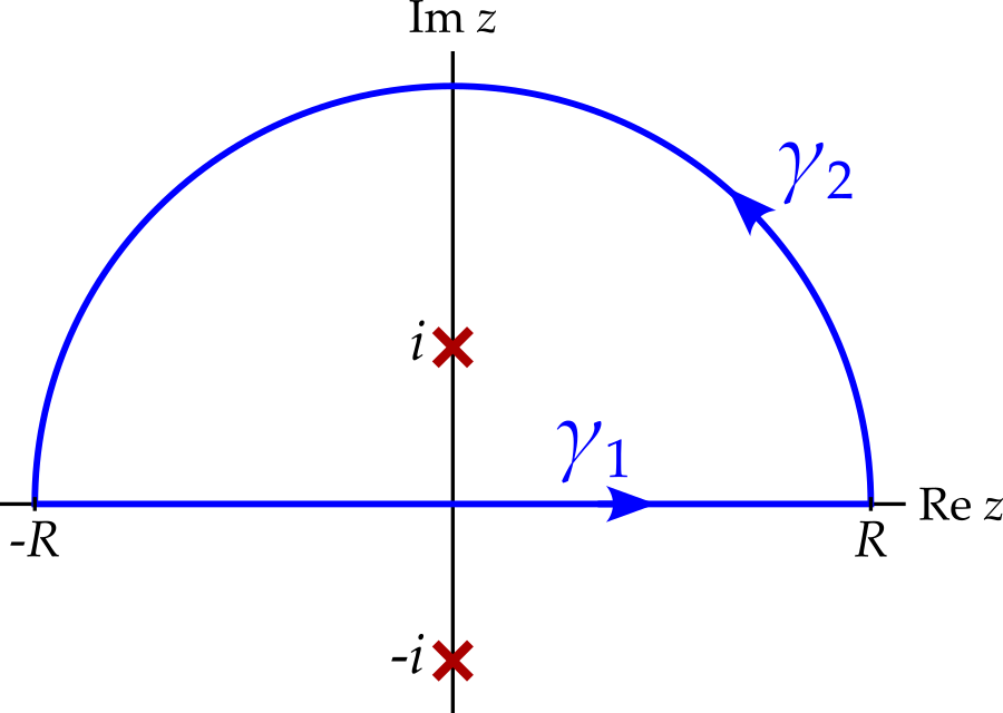
We have \[ \int_{\gamma_1} f(z)\,dz = \int_{-R}^R \frac{1}{x^2 + 1}\,dx \] and so \[ \lim_{R \rightarrow \infty}\int_{\gamma_1} f(z)\,dz = \int_{-\infty}^\infty \frac{1}{x^2 + 1}\,dx = 2I. \] Meanwhile, as |z| approaches infinity, the integrand approaches zero faster than \(1/z\). In other words \[ \lim_{\left|z\right| \rightarrow \infty}zf(z) = \lim_{\left|z\right| \rightarrow \infty}\frac{z}{z^2 + 1} = 0. \] Therefore, we know that \[ \lim_{R \rightarrow \infty}\int_{\gamma_2} f(z)\,dz = 0. \] Hence \[ \begin{aligned} I &= \frac{1}{2}\lim_{R \rightarrow \infty}\int_\gamma f(z)\,dz\\ &= \frac{1}{2}\int_\gamma \frac{1}{z^2 + 1}\,dz, \end{aligned} \]

where \(\gamma = \gamma_1 + \gamma_2\).⁶

⁶ Why can I drop the limit here? Well, this integral will always produce the same result, provided \(R\) is large enough to ensure that the contour goes around the pole.

Noticing that the contour only goes around one pole - that at \(z = i\). Calculating the residue, we get \[ \operatorname{Res}\left[\frac{1}{(z - i)(z + i)}\right]_i = \lim_{z \rightarrow i}\frac{1}{z + i} = \frac{1}{2i}. \] Applying the residue theorem, we get \[ I = \frac{1}{2}.2\pi.i\frac{1}{2i} = \frac{\pi}{2} \]

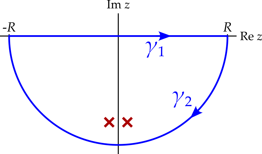
There are two things worth noticing here. Firstly, notice that the integrand approaches zero faster than \(1/z\) in the lower half plane two. Hence we could have closed the integral with a semi-circle there⁷.

⁷ The residue at \(z = -i\) is minus that at \(z = i\), but we get another minus sign due given that the contour is traversed clockwise. Hence we obtain the same result.

Secondly, if you know your standard integrals, you will notice that we could have performed this integral without complex analysis, i.e. \[ I = \int_0^\infty \frac{1}{x^2 + 1}\,dx = \left[\arctan x\right]_0^\infty = \frac{\pi}{2}. \] These results are consistent, which hopefully gives us some confidence in our methods. Of course, the complex analysis techniques are more useful when the integral cannot be calculated with standard methods.

9.5 Integrals with complex exponentials

Consider \[ I = \int_{-\infty}^\infty f(x)e^{iax}\,dx, \] where \(a \in \mathbb{R}\).⁸ For now, we will assume that \(a\) is positive and examine the case where \(a\) is negative later.

⁸ Yes, you should recognise this. It is the Fourier transform, that you will have seen in other classes.

We assume that

• \(f(z)\) is holomorphic in the upper half-plane, except for a finite number of isolated singularities.
• \(\displaystyle \lim_{\left|z\right| \rightarrow \infty} f(z) = 0\) for \(0 \leq \arg(z) \leq \pi\).

We can again employ the semi-circular contour show in figure 9.8.

Figure 9.8: Completing the contour in the upper half plane again.

Notice that the integrand, \(f(z)e^{iaz}\) approaches zero very quickly as the imaginary component of \(z\) becomes large and positive, since \[ \left|f(z)e^{iaz}\right| = \left|f(z)\right|e^{-a\operatorname{Im}z}. \tag{9.1}\] However, we cannot quite apply the results of section 9.4, because the integrand does not approach zero fast enough along the real axis.

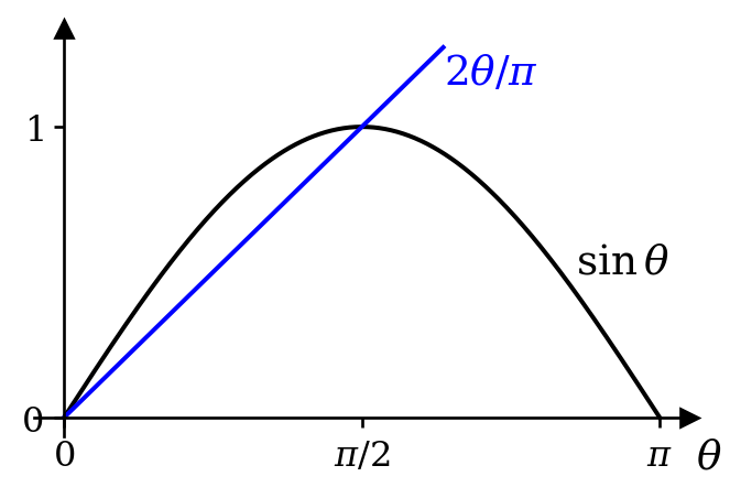
The integral along \(\gamma_1\) will approach \(I\) as \(R\) approaches infinity. Hence we would like the integral along \(\gamma_2\) to approach zero. On \(\gamma_2\) we set \(z = Re^{i\theta}\) and get \[ \begin{aligned} I_{\gamma_2} &= \int_{\gamma_2} f(z)e^{iaz}\,dz\\ &= \int_0^\pi f(Re^{i\theta})e^{ia\left(R\cos\theta + iR\sin\theta\right)}iRe^{i\theta}\,d\theta\\ &= \int_0^\pi f(Re^{i\theta})e^{iaR\cos\theta}e^{iR\sin\theta}iRe^{i\theta}\,d\theta\\ \end{aligned} \] Taking the modulus, we get \[ \begin{aligned} \left|I_{\gamma_2}\right| &= \left|\int_0^\pi f(Re^{i\theta})e^{iaR\cos\theta}e^{iR\sin\theta}iRe^{i\theta}\,d\theta\right|\\ &\leq \int_0^\pi \left|f(Re^{i\theta})e^{iaR\cos\theta}e^{-aR\sin\theta}iRe^{i\theta}\right|\,d\theta\\ &= R\int_0^\pi \left|f(Re^{i\theta})\right|e^{-aR\sin\theta}\,d\theta \end{aligned} \] We know that \(f(z) = f(Re^{i\theta})\) approaches zero as \(R\) approaches infinity, so for any \(\epsilon > 0\) we can make \(R\) large enough to ensure that \(\left|f(z)\right| < \epsilon\) along the contour. Hence \[ \left|I_{\gamma_2}\right| \leq \epsilon R\int_0^\pi e^{-aR\sin\theta}\,d\theta. \] This looks promising - as \(R\) becomes large, this integral should become small, but will it be small enough to cancel the factor of R? Notice that \[ \int_0^\pi e^{-aR\sin\theta}\,d\theta = 2\int_0^{\pi/2} e^{-aR\sin\theta}\,d\theta \] and that for \(\theta \in [0, \pi / 2]\) we have \(\sin\theta \geq 2\theta / \pi\).

Figure 9.9: Comparison of \(\sin\theta\) with \(2\theta / \pi\).

Hence \[ \begin{aligned} \left|I_{\gamma_2}\right| &= 2\epsilon R\int_0^{\pi/2} e^{-aR\sin\theta}\,d\theta\\ &\leq 2\epsilon R\int_0^{\pi/2}e^{-2aR\theta / \pi}\,d\theta\\ &= \frac{2\epsilon R}{2aR\pi}(1 - e^{aR})\\ &= \frac{\pi\epsilon}{a}(1 - e^{aR}). \end{aligned} \] Since \(\epsilon\) can be made as small as we wish by increasing \(R\), we see therefore that \[ \lim_{R \rightarrow \infty}I_{\gamma_2} = 0. \] This result is known as Jordan’s lemma. This now means that \[ I = \int_{-\infty}^\infty f(x)e^{iax}\,dx = \oint_\gamma f(z)e^{iaz}\,dz, \] which can be evaluated using the residue theorem. Here, \(\gamma = \gamma_1 + \gamma_2\).

What happens when \(a\) is negative? Now equation 9.1 shows that, for negative \(a\), \(f(z)e^{iaz}\) approaches zero very quickly as the imaginary component of \(z\) becomes large and negative and so we would close the contour in the lower half-plane.

Figure 9.10: Completing the contour in the lower half plane.

Example 9.5 \[ I = \int_0^\infty \frac{\cos x}{x^2 + 1}\,dx. \] We use the definition of cosine, \(\cos x = (e^{ix} + e^{-ix}) / 2\) to get \[ I = \frac{1}{2}\int_0^\infty \frac{e^{ix}}{x^2 + 1}\,dx + \frac{1}{2}\int_0^\infty \frac{e^{-ix}}{x^2 + 1}\,dx. \] A change of variables from \(x\) to \(-x\) in the second integral gives us \[ \begin{aligned} I &= \frac{1}{2}\int_0^\infty \frac{e^{ix}}{x^2 + 1}\,dx + \frac{1}{2}\int_{-\infty}^0 \frac{e^{-ix}}{x^2 + 1}\,dx\\ &= \frac{1}{2}\int_{-\infty}^\infty \frac{e^{ix}}{x^2 + 1}\,dx \end{aligned} \] and we have the integral in the correct form.

We now analytically continue, so that the integrand becomes \[ \frac{e^{iz}}{z^2 + 1} = f(z)e^iz, \] where \(f(z) = 1 / (z^2 + 1)\) approaches zero as \(\left|z\right|\) approaches infinity, regardless of the direction taken. Moreover, \(e^iz\) shrinks exponentially towards zero as the imaginary part of \(z\) gets large and positive, so we close the contour in the upper half-plane.

Figure 9.11: Completing the contour in the upper half plane yet again.

Using Jordan’s lemma, the integral along \(\gamma_2\) approaches zero, while that along \(\gamma_1\) approaches (twice) the integral we want. Calculating the integral around the entire contour, we need the residue at \(z = i\). \[ \operatorname{Res}\left[\frac{e^{iz}}{(z + i)(z - i)}\right]_i = \lim_{z \rightarrow i}\frac{e^{iz}}{z + i} = \frac{1}{2ie}. \] Hence \[ I = \frac{1}{2}\oint_{\gamma}\frac{e^{iz}}{z^2 + 1}\,dz = \frac{1}{2}.2\pi i.\frac{1}{2ie} = \frac{\pi}{2e}. \]

9.6 Integrals of multivalued functions

We conclude by looking at an example of integrating a multivalued function. Here we will not only need to determine how to close the contour, but also where to place the branch cut⁹.

⁹ While, technically speaking, an integration contour can cross a branch cut, this immediately rules out the use of Cauchy’s theorem and the residue theorem, since some of the branch cut must be inside the contour. It therefore makes sense to place the contour and the branch cut such that they do not meet.

¹⁰ For clarity, I will draw it a little above the real axis, for reasons that will soon become clear.

Consider \[ I = \int_0^\infty \frac{x^p}{x^2 + 1}\,dx, \] where \(0 < p < 1\). We start by drawing the initial contour, \(\gamma_1\), from \(\epsilon\) to \(R\) along the positive real axis¹⁰. (To be safe, we avoid the branch point at \(z = 0\).) The integral we want is now the limit, as \(R \rightarrow \infty\) and as \(\epsilon \rightarrow 0\), of the integral along \(\gamma_1\). \[ I = \lim_{\substack{R \rightarrow \infty\\\epsilon\rightarrow 0}} \int_{\gamma_1} \frac{z^p}{z^2 + 1}\,dz. \] We write \[ f(z) = \frac{z^p}{z^2 + 1} \] and note that this approaches zero faster than \(1/z\) as \(\left|z\right| \rightarrow \infty\). Hence the integral along any circular arc starting at \(R\) and centred at zero will approach zero as \(R \rightarrow \infty\). It therefore seems to make sense to continue the contour along such an arc, which we will label \(\gamma_2\).

Figure 9.12: Starting the contour.

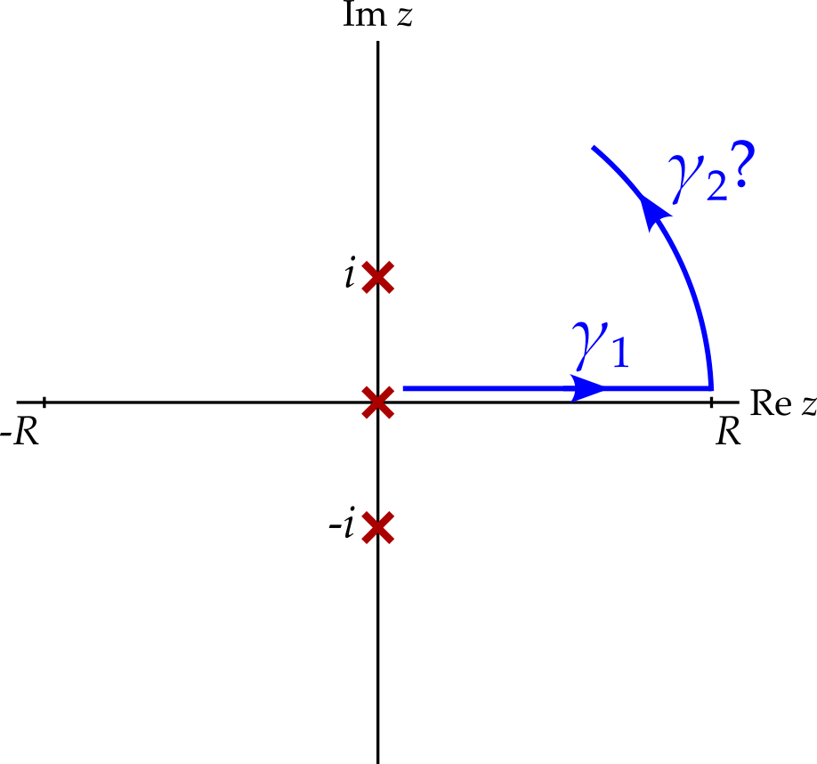
We now have two problems. How should we arrange for the contour to return to the start point? Where should the branch cut go?

We can continue around the circular arc for as long as we wish - the integral along the arc can always be made to approach zero, by increasing \(R\). The return to the start point, however, cannot easily be arranged so as to make its contribution to the integral equal zero. Instead, we will arrange for it to produce an integral related to \(I\) in a simple way.

One way to do this is to let \(\gamma_2\) go almost all the way around the circle until it returns to a point just below \(R\). The third part of the contour, \(\gamma_3\) will then lie just below \(\gamma_1\) but be traversed in the opposite direction.

But doesn’t this just cancel the integral along \(\gamma_1\)? And where does the branch cut go? Since we do not want the branch cut to cross the contour, we only have one option - we place it along the positive real axis, constraining the argument of \(z\) to be in \([0, 2\pi)\). The resulting discontinuity also ensures that the values of \(f(z)\) differ between neighbouring points on contours \(\gamma_1\) and \(\gamma_3\).

Figure 9.13: Continuing the contour.

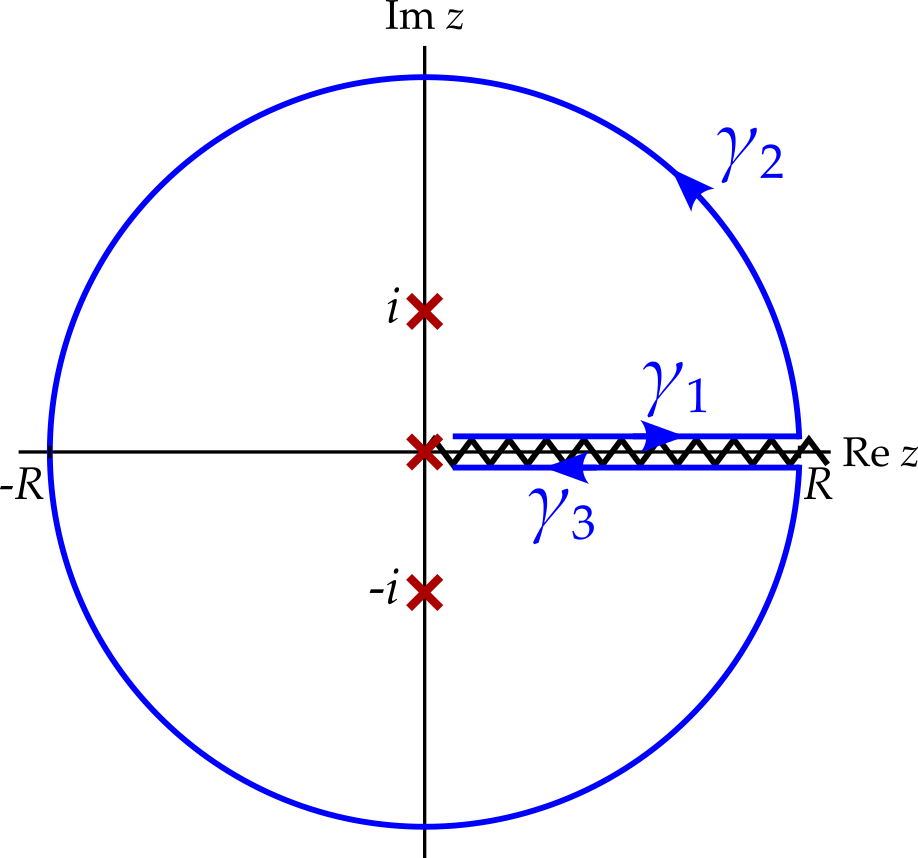
Let’s evaluate the integral along \(\gamma_3\), being careful to write \[ z = xe^{2\pi i}, \] i.e. to insist that the argument of \(z\) is \(2\pi\) on this contour¹¹. Hence \[ \int_{\gamma_3} f(z)\,dz = \int_R^\epsilon \frac{x^pe^{2p\pi i}}{x^2 + 1}\,dx = -e^{2p\pi i}\int_\epsilon^R \frac{x^p}{x^2 + 1}\,dx \] and so \[ \lim_{\substack{R \rightarrow \infty\\\epsilon\rightarrow 0}} \int_{\gamma_3} \frac{z^p}{z^2 + 1}\,dz = -e^{2p\pi i}I. \]

¹¹ Actually, \(\arg{z}\) is very slightly less than \(2\pi\), but we will take the limit \(\arg{z} \rightarrow 2\pi\).

Finally, we complete the contour by adding a circle, \(\gamma_4\), of radius \(\epsilon\) around the origin. The creates the ‘keyhole contour’.

Figure 9.14: The keyhole contour.

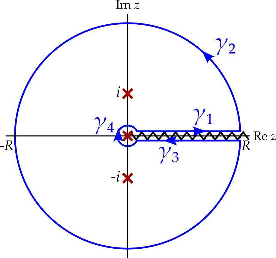
It remains for us to show that the integral on \(\gamma_4\) approaches zero as \(\epsilon\) approaches zero. This certainly seems reasonable, since the both the integrand and the length of the contour approach zero. Indeed, provided \(\epsilon < 1/2\), we have \[ \left|\frac{z^p}{z^2 + 1}\right| = \frac{\left|z^p\right|}{\left|z^2 + 1\right|} \leq \frac{1}{3/4} = \frac{4}{3}, \] for all \(z\) on \(\gamma_4\). Hence, using the useful result of section 6.2.1, we have \[ \left|\int_{\gamma_4}f(z)\,dz\right| \leq 2\pi\epsilon.\frac{4}{3}, \] which approaches zero as \(\epsilon\) approaches zero.

To summarise, if we taking the limit as \(R \rightarrow \infty\) and \(\epsilon \rightarrow 0\), then we get \[ \begin{aligned} \oint_\gamma f(z)\,dz &= \oint_{\gamma_1} f(z)\,dz + \oint_{\gamma_2} f(z)\,dz + \oint_{\gamma_3} f(z)\,dz + \oint_{\gamma_4} f(z)\,dz\\ &= I + 0 - e^{2p\pi i}I + 0\\ &= (1 - e^{2p\pi i})I. \end{aligned} \]

We now use the residue theorem to calculate this integral. To do this we need the residues of the poles at \(z_1 = i\) and \(z_2 = -i\) and when calculating these, we must remember to use values for the argument of \(z\) that lie in \([0, 2\pi)\) when calculating \(z^p\). Hence \[ z_1 = i = e^{\pi i / 2} \] and \[ z_2 = -i = e^{3\pi i / 2}, \] not $e^{-i / 2} Calculating the residue at \(z_1 = i\), we get \[ \begin{aligned} \operatorname{Res}\left[\frac{z^p}{z^2 + 1}\right]_i &= \lim_{z \rightarrow i}\frac{(z - i)z^p}{z^2 + 1} = \lim_{z \rightarrow i}\frac{z^p}{z + i}\\ &= \frac{(e^{\pi i/2})^p}{2i} = \frac{e^{p\pi i/2}}{2i}. \end{aligned} \] Meanwhile \[ \begin{aligned} \operatorname{Res}\left[\frac{z^p}{z^2 + 1}\right]_{-i}i &= \lim_{z \rightarrow -i}\frac{(z + i)z^p}{z^2 + 1} = \lim_{z \rightarrow -i}\frac{z^p}{z - i}\\ &= \frac{(e^{3\pi i/2})^p}{-2i} = -\frac{e^{3p\pi i/2}}{2i}. \end{aligned} \]

So, finally we have \[ \begin{aligned} I &= \frac{2\pi i}{1 - e^{2p\pi i}}.\frac{1}{2i}\left(e^{p\pi i/2} - e^{3p\pi i/2}\right)\\ &= \pi\frac{e^{p\pi i/2} - e^{3p\pi i/2}}{1 - e^{2p\pi i}}. \end{aligned} \] Multiply both numerator and denominator by \(-e^{p\pi i}\) to get \[ \begin{aligned} I &= \pi\frac{e^{p\pi i/2} - e^{-p\pi i/2}}{e^{p\pi i} - e^{-p\pi i}}\\ &= \pi\frac{\sin(p\pi / 2)}{\sin(p\pi)}\\ &= \frac{\pi}{2\cos(p\pi / 2)}. \end{aligned} \]